Code organisation

05 December, 2023

organisation of the code

Main program termsProgram

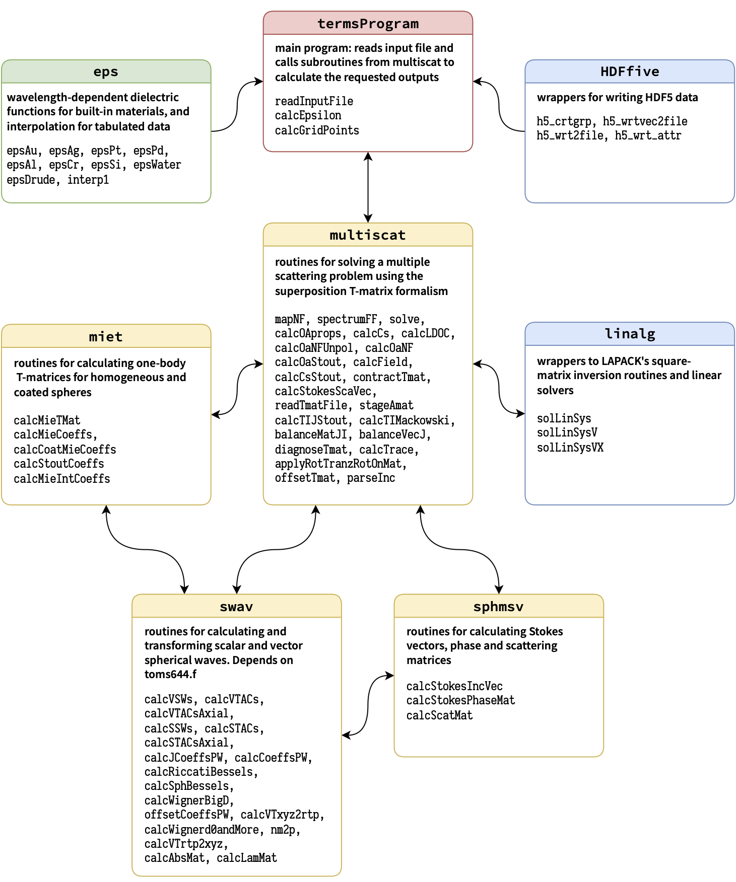
termsProgram is the main module, with subroutines listed below; it reads the keywords and their corresponding values in the input file and then calls different subroutines of multiscat module for the calculation of requested outputs.

• readInputFile(inputfile)
  Reads the input file containing specific keywords and the corresponding parameter values.

• errorParsingArguments(keyword)
  If there is an error with the parameter values assigned to a keyword, this subroutine informs the user and stops the program.

• calcEpsilon()
  Updates the escat array storing the relative dielectric function(s) for each scatterer evaluated at the specified wavelengths.
  escat is an array for which the number of rows, columns and the 3\(^{rd}\) dimension correspond to the number of shells, scatterers, and wavelengths, respectively.

• calcGridPoints(points)
  For a near-field calculation, this subroutine calculates the grid points based on the number of steps, lower and upper values along the desired axes.
  points(3, nGridPoints) is an in/output matrix storing the cartesian coordinates \((x,y,z)\) of the grid points.

• sentence2words(sentence, words, nwords_)
  Reads each line of the input file as a sentence and splits it into space-separated words.
  sentence, words are in/output character arrays, and nwords_ is an optional output integer containing the number of words in the sentence.

• dumpNFs2TXTFile(filename, incidences, Epower, wavelen, work, Ef, p_label)
  Exports electric and magnetic near fields into a plain text file. filename is the name of the text file. incidences, Epower, wavelen, work are the incidence angles, selected power for mapping fields, wavelength, and near-field quantities, respectively. Ef is a logical flag which selects either electric field or magnetic field. p_label is an integer array indexing the position of each grid point, whether it is inside the surrounding medium or a particle, and in which layer.

• dumpNFs2HDF5File(fname, groupname, filename, incidences, Epower, wavelen, work, p_label) Exports electric and magnetic near fields into a HDF5 file. filename, fname, groupname are the names of the HDF5 file, group, and subgroup name, respectively. incidences, Epower, wavelen, work are the incidence angles, selected power for mapping fields, wavelength, and near-field quantities, respectively. Ef is a logical flag which selects either electric field or magnetic field. p_label is an integer array indexing the position of each grid point, whether it is inside the surrounding medium or a particle, and in which layer.

• countLines(filename) result(nlines)
  Counts lines in a text file.

multiscat module

This module consists of a mix of high-level, core, low-level and supplementary routines for solving a multiple scattering problem using the T-matrix formalism. We list below the subroutines of the multiscat module with a brief explanation. A list of common arguments and their brief description is at the end of this section. The other arguments are explained after each subroutine.

• mapNF(ncut, wavelen, inc,ehost, geometry, scheme, tfiles_, escat_, nselect_, verb_, noRTR_, dump_oaE2, dump_oaB2, field, Bfield, N_OC, orAvextEB_int, oa_ldoc, p_label)
  Calculates the electric and magnetic near fields, and normalised optical chirality (\(\overline{\mathscr{C}}\)) for a multiple scattering problem, for different incidence directions and wavelengths, as well as the orientation-averaged value of external \(\langle|\mathbf{E}|^2\rangle, \langle|\mathbf{B}|^2\rangle\) and \(\langle\overline{\mathscr{C}}\rangle\). escat_, tfiles_, nselect_, verb_, noRTR_ are optional inputs. dump_oaE2, dump_oaB2 are logical flags selecting whether the orientation-averaged values \(\langle|\mathbf{E}|^2\rangle\) and \(\langle|\mathbf{B}|^2\rangle\) will be calculated, respectively.

• spectrumFF(ncut, wavelen, ehost, geometry, scheme, escat_, tfiles_, nselect_, noRTR_, verb_, sig_oa_, sig_, sig_abs_, jsig_abs_oa)
  Calculates cross-section spectra for (multiple) fixed orientations, partial absorptions, and orientation-averaged cross-sections for a particle cluster. T-matrices for individual scatterers are either constructed using Mie theory or read from an optional argument tfiles_. escat_, tfiles_, nselect_, verb_, noRTR_ are optional inputs. jsig_abs_oa contains the orientation-averaged absorption cross-section of each particle (valid for homogeneous spheres only, at present).

• solve(wavelen, ehost, geometry, nselect_, scheme_, verb_, noRTR_, TIJ, cJ_, cJint_, csAbs_, ierr_ )
  This routine is the crux of terms and solves a given multiple scattering problem by operating in a specified scheme. TIJ is an in/output argument, cJ_, cJint_, csAbs_ are optional in/output arguments, nselect_, scheme_, verb_, noRTR_ are optional inputs, and ierr_ is an optional output. TIJ (\(l_{max}\times \text{nscat}\), \(l_{max}\times\text{nscat}\)) as the input argument stores the T-matrix of nonspherical particles as the diagonal blocks of the matrix, or dielectric values of different shells for spherical particles as the diagonal elements of the matrix. nscat is the number of scatterers. This subroutine updates and returns TIJ for the whole system as the output. cJ_(nscat x l_{max}, 2, nfi) as the input argument contains details of the incident field and as a output argument contains incident plane wave coefficients in the first column and scattering coefficients in the second column. nfi is the number of incident angles. cJint_(nscat x l_{max}, 4, 2): contains the regular and irregular field coefficients for each concentric region inside spherical scatterers. csAbs_(nscat,4): contains absorption cross section inside each shell of each spherical scatterer.

• stageAmat(scatXYZ, scatMiet, rtr, right_, balance_, verb_, A, Tmats_)
  Stages a pre-staged matrix \(A\).
  A (l_{max} x nscat, l_{max} x nscat): an in/output matrix, which must contain 1-body T-matrices in the diagonal blocks on input and is a pre-staged matrix on the output; right_, balance_, verb_ are optional inputs; Tmats_(l_{max}, l_{max}, nscat): an optional output matrix which contains the 1-body T-matrix of each particle. balance_: a logical input argument which determines whether balancing is applied or not.

• calcTIJStout(scatXYZ, scatMiet, rtr, TIJ)
  Calculates the scatterer-centred T-matrix using the recursive scheme presented in Stout. TIJ is an in/output argument. TIJ(l_{max} x nscat, l_{max} x nscat) as the input argument stores the T-matrix of nonspherical particles as the diagonal blocks, or dielectric values of different shells for spherical particles as diagonal blocks.

• calcTIMackowski(scatXYZ, scatMiet, rtr, TIJ)
  Calculates the cluster’s T-matrix using Mackowski & Mishchenko’s formulation. TIJ is an in/output argument. TIJ(l_{max} x nscat, l_{max} x nscat) as the input argument stores the T-matrix of nonspherical particles as the diagonal blocks, or dielectric values of different shells for spherical particles as diagonal blocks. The output TIJ is the scatterer-centred T-matrices calculated using Mackowski & Mishchenko’s scheme.

• balanceMatJI(j, jregt, iregt, i, rev_, mnq_, Mat)
  Performs balancing on a matrix (Mat) using two weights (indexed by \(j\) and \(i\)). Mat is here taken as relating two vectors of VSWF coefficients, \(c_j\) (centred at \(j\)) and \(c_i\) (centred at \(i\)), such that \(c_j = \text{Mat}\, c_i\). Logical inputs jregt and iregt specify whether \(c_j\) and \(c_i\) are regular or not. Mat is an in/output argument.

• balanceVecJ(j, jregt, rev_, Vec)
  Performs balancing on a single vector (V) with a weight indexed by \(j\). V corresponds here to the VSWF coefficients of particle \(j\). Vec is an unbalanced/ balanced vector as the in/output argument. j specifies the scatterer.

• calcCsStout(scatXYZR, aJ, fJ, nmax2_, tol_, verb_, sig)
  Calculates the extinction, scattering and absorption cross-sections from the incident and scattered coefficients using the Stout formulae. nmax2_, tol_, verb_ are optional inputs and sig is an in/output matrix.

• calcCs(scatXYZR, inc, fJ, nmax2_, tol_, verb_, sig)
  Calculates the extinction, scattering and absorption cross-sections from the incident and scattered coefficients which are collapsed to the common origin. Depending on the dimension of the sig, each cross-section is either just a total sum, or resolved into contributions from the multipole orders. inc: a vector of incidence angles.

• calcOAprops(Tmat, rtol_, sigOA, verb_)
  Calculates orientation-averaged cross-sections and circular dichroism (CD) by transforming the T-matrix (Tmat) from "parity" (M–N) basis to "helicity" (L–R) basis, following Ref. . rtol_ is an optional input, verb_ is an optional output, and sigOA is an in/output matrix containing orientation-averaged cross-sections and CD in each column for \(n=1, \dots, n_{max}\).

• contractTmat(Tin, scatXYZR, rtr, mack_, Tout, verb_)
  Combines the scatterer-centred T-matrices into a common origin; the output will be the collective T-matrix (Tout). verb_ is an optional in/output, mack_ is an optional logical input to calculate the collective T-matrix based on Mackowski & Mishchenko’s scheme.

• alphaTensor(T, Alpha)
  Conversion of \(l\leq 3\) spherical multipoles of the T-matrix \(T\) into cartesian multipoles (tensor Alpha), following formulas for ‘Higher-Order Polarizability Tensors’ in Mun. This function is called when the keyword DumpCollectiveTmatrix is present, and outputs a file alpha_col.txt in the working directory.

• diagnoseTmat(mode_, verb_, Tmat)
  Determines the value of \(n \leq n_{max}\) when \(\operatorname{Tr}(\Re{(\text{Tcol})})\) converges to \(\text{rtol\_G}:=10^{-\text{ncut(3)}}\). If mode_ \(> 0\), also tests for the general symmetry, which applies to all T-matrices. (See equation 5.34 on p. 121 of Mishchenko).

• calcOaStout(TIJ, scatXYZ, verb_, sigOA, cdOA_, jAbsOA)
  Calculates the orientation-averaged extinction and scattering cross-sections defined in equations 44 and 47 of Stout. The absorption cross-section is then deduced as the difference. TIJ is the collective T-matrix, sigOA(3) contains orientation-averaged extinction and scattering cross-sections, and cdOA_ is an optional output containing the corresponding values of

  400. jAbsOA: contains the orientation-averaged absorption cross-section for each particle.

• applyRotTranzRotOnMat(vtacs, bigdOP, rightOP, mat)
  Performs the factorised translation of T-matrices when changing origin. Instead of a single multiplication of a T-matrix by a dense matrix containing the general translation-addition coefficients, this routine executes three multiplications by sparse matrices representing 1) a rotation, 2) a translation along the z-axis; and 3) an inverse rotation. This is meant to be more efficient when high multipole orders are included.
  vtacs(2x pmax,2 x pmax): axial VTACs with \((m,n,q)\) indexing, bigdOP(pmax, pmax): optional input for rotation, rightOP: an optional logical input argument for applying the product from the right. mat: a non/translated matrix as the in/output.

• calcField(r, geometry, ipwVec, ipwE0, scaCJ, intCJreg_, intCJirr_, scatK_, verb_, reE, imE, reB, imB, reE_sca,imE_sca, reB_sca,imB_sca, p_label)
  Calculates the electric and magnetic near-field values at the determined grid points.
  r: a matrix containing the coordinates of the grid points; ipwVec(3),ipwE0(3): contain the wavevector and amplitude of the incident field, respectively; scaCJ: a vector containing scattering coefficients, intCJreg_, intCJirr_: contain the regular and irregular parts of the incident field coefficients transformed to the origin of each particle, respectively, scatK_ is the wavenumber in the host medium, and reE, imE, reB, imB, reE_sca,imE_sca, reB_sca,imB_sca: contain real(re) and imaginary(im) parts of the total electric (E) and magnetic (B) fields and the scattered field values at the grid points.

• dumpTmat(tmat, filename, lambda, eps_med, tol_, verb_)
  Routine for dumping the collective T-matrix (tmat) to a file in the format:

  s, s’, n, n’, m, m’, T_re, T_im

  filename is an argument of type character corresponding to the name of the output file; lambda: the value of wavelength; eps_med: the dielectric value of the host medium.

• dumpMatrix(mat, ofile, tolOP, verb_)
  Outputs matrix mat to a desired optional tolerance (tolOP). ofile: the name of the output file.

• offsetTmat(off, miet, rtr, right, bigD_, useD_, balJI_, Tmat)
  Offsets the supplied T-matrix Tmat by off, which can be either a square matrix of VTACs or a (note: complex!) displacement vector \(k\mathbf{r}\)(3) from which VTACs will be generated. Regular or irregular VTACs will be generated depending on whether \(k\mathbf{r}\)(3) is purely real or purely imaginary. If the logical input miet is true, Tmat will be treated as diagonal. If the logical input rtr is true, then offsetting will be based on factorised translation. If the logical input right is true, then offsetting will be done by post-multiplying Tmat from the right. balJI_ triggers balancing of the VTACs and the T-matrices individually, before offsetting, but currently works only without factorised translation.

• readTmatFile(filename, unit, wavelen, verb_, Tmat)
  Reads a T-matrix from the input file (filename) and import it into the matrix Tmat. unit: an integer indexing the name of the T-matrix file. wavelen is the value of the wavelength.

• parseInc(inc, verb_, inc_dirn, inc_ampl)
  Calculates the amplitude and direction vector of the incident plane wave based on the input Euler angles (\(\alpha, \beta, \gamma\)). inc_dirn and inc_ampl are vectors containing the wavevector and amplitude of the incident electric field in cartesian coordinates, respectively. inc is a vector consisting of polarisation type and Euler angles of the incidence direction.

• calcStokesScaVec(sca_angles, inc2, ncut, wavelen, ehost, geometry, scheme, tfiles_, escat_, nselect_, noRTR_, verb_, StokesPhaseMat, StokesScaVec, diff_sca)
  Calculates the Stokes phase matrix (StokesPhaseMat), Stokes scattering vector (StokesScaVec), and differential scattering cross-sections (diff_sca).
  sca_angles is a matrix of desired scattering angles; if it is not specified in the input file, they are taken equal to the incidence angles. inc2 is a matrix containing incidence angles.

• calcLDOC(Ef, Bf, verb_, N_OpC)
  Calculates the normalised optical chirality (\(\overline{\mathscr{C}}\)) relative to the optical chirality of circularly polarised light. Ef, Bf, and N_OpC are matrices containing the electric and magnetic field, and \(\overline{\mathscr{C}}\) values at the grid points, respectively.
  

• calcOaNFUnpol(r, geometry, TIJ, lambda, ehost, escat, p_label, verb_, orEB2)
  Calculates the orientation average of the total external electric and magnetic field intensities. r is a matrix containing the cartesian coordinates of the grid points. TIJ is the scatterer-centred T-matrix of the cluster. orEB2 is a vector containing the value of orientation-averaged external electric and magnetic field intensities at the grid points.

• calcOaNF(pol_type, r, geometry, TIJ, Oa_OC, ehost, p_label, scatK_, verb_, Oa_EB2)
  Calculates the orientation average of normalised optical chirality \(\langle\overline{\mathscr{C}}\rangle\), and near field intensities \(\langle |\mathbf{E}_\mathrm{tot}(\it{k}\mathbf{r})|^2\rangle\), \(\langle |\mathbf{B}_\mathrm{tot}(\it{k}\mathbf{r})|^2\rangle\) for circularly polarised incident light. pol_type is the polarisation type, r is a matrix containing the cartesian coordinate of the grid points. TIJ is the scatterer-centred T-matrix of the structure.

• calcTrace(TRANSA, TRANSB, A, B, tr)
  Calculates the trace of a product of two matrices, op(A)*op(B). The input characters TRANSA and TRANSB determine the operation op, following the convention of blas’ gemm. Specifically, op = ’N’ corresponds to \(\mathtt{op(A) = A}\) (no operation), whereas op = ’C’ corresponds to \(\mathtt{op(A) = A^\dagger}\).

• RotMatX(ang) result(rotMat)
  Calculates a rotation matrix along the x axis using input argument angle(ang).

• RotMatY(ang) result(rotMat)
  Calculates a rotation matrix along the y axis using input argument angle(ang).

• RotMatZ(ang) result(rotMat)
  Calculates a rotation matrix along the z axis using input argument angle(ang).

• rotZYZmat(angles) result(mat)
  Calculates rotation matrix mat for ZY’Z’, using the Euler angles=(\(\alpha,\beta,\gamma\))

List of common arguments

• acs_int_: a matrix containing partial internal absorption inside each scatterer and for each shell.

• aJ(\text{nscat}\times l_{max}), fJ(\text{nscat}\times l_{max}): contains incident and scattering coefficients.

• Bfield: contains the real and imaginary parts of the magnetic near field at the specified grid points, wavelengths, and incidence.

• ehost: a vector of dielectric permittivity of the host medium at specified wavelengths.

• escat_(nscat, 4, size(wavelen)): depending on the number of wavelengths, it is a 2D or 3D array of dielectric values for each scatterer, for each shell and wavelength.

• field: contains the real and imaginary parts of the electric near field at the specified grid points, wavelengths, and incidence.

• geometry: a matrix containing physical information of different scatterers such as centre, dimensions and direction.

• ierr_: an integer value (0 or 1 or 2); 0 indicates solving was successful, 1 means there is an error in processing arguments, and 2 means an error in prestaging, staging, or solving/inverting \(Ax=b\).

• iregt: logical input, specifies whether vectors are regular or not.

• jregt: logical input, specifies whether vectors are regular or not.

• mnq_: an optional logical argument which is false by default, but if true will change the indexing convention from (q,n,m) to (m,n,q), which is used to make the z-axial VTACs block-diagonal. Note that index \(q\) corresponds to \(s\) in this user guide.

• ncut: a vector in the form [\(n_1\), \(n_2\), tol], which contains the values corresponding to the keyword "MultipoleCutoff". Default values: \([8, 8, -8]\).

• nmax2_: an integer value equals to ncut(2).

• noRTR_: an optional input with logical value .true. or .false. for the keyword DisableRTR. Default: .false..

• nselect_: an optional input matrix which includes information about multipole selection for different scatterers.

• oa_ldoc (\(\text{npts}\times 4\times \text{nwavelen}\)): contains the orientation averaged value of \(\overline{\mathscr{C}}\) at different grid points and wavelengths.

• orAvextE_int(\(\text{npts}\times \text{nwavelen}\)): contains the orientation averaged electric field intensity values at different grid points and wavelengths.

• p_label: a matrix determining the position of each grid point, whether it is inside the surrounding medium or particles, and in which layer.

• rev_: an optional logical input which is false by default; triggers the reverse of balancing – "unbalancing".

• right_: a logical input. There are two ways for obtaining the TIJ matrix. This argument determines whether the product is taken from the left or from the right.

• rtr: a logical input that is the reverse of noRTR_.

• scatMiet(nscat): a logical vector with .true. and .false. values, determining whether a scatterer is spherical or not.

• scatXYZ(3,nscat): a matrix containing the cartesian coordinates (in lab frame) of the particle’s centre.

• scatXYZR(4,nscat): a matrix containing the cartesian coordinates (in lab frame) and the radius of the smallest circumscribed sphere of each particle.

• scheme, scheme_: an integer value specifying the selected scheme.

• sig_: a matrix containing cross-sections (Extinction, Scattering, Absorption) for different polarisation(s), wavelength(s), and incidence(s).

• sig_abs_(\(4\times \text{nscat}\times 4\times \text{nwavelen}\times \text{nfi}\)): a 5D array containing absorption cross-sections inside each shell for each scatterer for 4 Jones vectors, different wavelengths and different incidence directions.

• sig_oa_(\(6\times \text{n}\times \text{nwavelen}\)): a matrix consisting of orientation-averaged cross-sections and CD at different wavelengtha. The first column gives the values for \(n_{max}\) and other columns contain values for different value of \(n=1, \dots, \text{ncut(2)}\).

• tfiles_: a matrix of character type, includes the T-matrix filename and filepath for non-spherical scatterers.

• tol_, rtol_: a real value rtol_G = 10^{\textbf{ncut(3)}}.

• N_OC: contains \(\overline{\mathscr{C}}\) at the specified grid points, wavelengths, and incidence.

• verb_: an integer variable containing the verbosity value (\(\in [0,1,2,3]\)) (the default value is 1).

• wavelen: a vector of specified wavelength(s).

miet module

This module contains routines for calculating one-body T-matrices (currently limited to spherical scatterers, using Mie theory).

• calcMieTMat(x, s, zeropad_, tmat)
  Calculates the diagonal T-matrix of a spherical scatterer for a given size parameter x=kR, relative refractive indices (\(s = k_{in}/k_{out}\)); zeropad_=nmax maximum value of the multipole index inferred from tmat’s dimensions.

• calcMieCoeffs(x, s, gammas, deltas)
  Calculates the Mie coefficients for a spherical scatterer as defined by equations H.46 and H.47 of Ref. . The coefficients are interpreted as magnetic and electric susceptibilities (\(\Gamma_n\) and \(\Delta_n\), respectively) of the scattered field. Note the relation to standard Mie coefficients: \(a_n = -\Delta_n\) and \(b_n = -\Gamma_n\).

• calcCoatMieCoeffs(x, s, gammas, deltas)
  Calculates the Mie coefficients for a coated sphere based on the equations H.110 and H.113 of Etchegoin and Le Ru.

• calcStoutCoeffs(x, rri, nmax, Cn, Dn)
  Calculates the Cn,Dn coefficients as defined by equation (50) in Stout. These coefficients are used to calculate absorption cross-sections. rri is the relative refractive index, nmax is the maximum value of the multipole index.

• calcMieIntCoeffs(a, k, scaCoeffs, intCoeffsReg, intCoeffsIrr, csAbs)
  Calculates the regular and irregular VSWF coefficients for the field inside each concentric region of a (layered) Mie scatterer. The formulae are based on Eqs. H.117–H.123 of Etchegoin and Le Ru. a, k, and scaCoeffs are vectors of the radius of the concentric interfaces, relative refractive index, and scattered field coefficients for the host medium, respectively. intCoeffsReg and intCoeffsIrr are matrices of regular and irregular field coefficients for each concentric region inside the scatterers and csAbs contains the partial absorptions calculated using equation (29) in Mackowski.

swav module

This module contains routines for calculating and transforming scalar (SSWs) and vector spherical waves (VSWFs). It depends on Amos (toms644.f) to calculate spherical Bessel and Hankel functions using recurrence. In order to limit redundancy, parameter definitions are renewed only where they are changed.

• calcVTACs(r0, k, regt, vtacs)
  Calculates the irregular (if regt=.false.) or the regular (if regt=.true.) vector translation-addition coefficients for a given kr0.
  r0 is a relative position vector, k is the wavenumber, regt is a logical argument which determines the type: regular or irregular, and vtacs(1:2*pmax,1:2*pmax) is the input/output array.

• calcSTACs(r0, k, pmax, regt, scoeff)
  Calculates the scalar translation-addition coefficients.(\(\alpha_{nu,mu;n,m}\) or \(\beta_{nu,mu;n,m}\)). The output corresponds to the scalar translation-addition coefficients \alpha(irregular, for regt=.false.) or \beta(regular, for regt=.true.).
  pmax is a maximal composite index and scoeff(0:pmax,0:pmax) is the coefficients matrix.

• calcVTACsAxial(r0, k, pmax, regt, flip, mqn_, vtacs)
  Calculates the irregular (if regt=.false.) or the regular (if regt=.true.) vector translation-addition coefficients for a given kr0, along the z-axis.
  r0 is the z-axial displacement distance, flip is a logical argument, mqn_ is a logical argument for changing from qnm to mqn indexing, and vtacs(1:2*pmax,1:2*pmax) is the matrix of coefficients.

• calcSTACsAxial(r0, k, pmax, regt, flip, stacs)
  Calculates the normalised scalar translation-addition coefficients along the z-axis for a given kr0.
  r0 is a displacement distance and stacs(0:pmax,0:pmax) is the coefficients matrix corresponding to \(\alpha\) (irregular, for regt=.false.) or \(\beta\).

• calcVSWs(r, k, pmax, regt, cart, waves, wavesB)
  Calculates (at r) the normalised vector spherical waves, \(M_{nm}\) and \(N_{nm}\) for evaluation of electric and magnetic fields
  r(3) is the cartesian coordinate of a point in 3D; cart is a logical argument which triggers conversion to cartesian coordinates; waves(2*pmax,3) contains elements (\(M_{nm}\) and \(N_{nm}\)) of the abstract column vector defined in Eq. B1 of Ref. and wavesB(2*pmax,3) is similar to waves, only swapping the position of \(M_{nm}\) and \(N_{nm}\) and multiplying by \(-ik\) for calculation of the magnetic field.

• calcSSWs(xyz, k, pmax, regt, psi)
  Calculates (at xyz) the scalar spherical waves \psi_{nm}.
  xyz is the cartesian coordinates of a point in 3D; psi(0:pmax) contains elements of the spherical waves \psi_{nm} as defined by equation 13a in Chew.

• calcJCoeffsPW(ipwE0, kVec, xyz, ipwCoeffsJ)
  Translates the supplied ipwCoeffs coefficients to different centres for an incident plane wave.
  ipwE0(3) is the incident plane wave’s amplitude vector, kVec(3) is the incident wave vector, xyz(3,nscat) is a matrix containing the centre of different scatterers, and ipwCoeffsJ(\(\text{nscat} \times \text{lmax}\)) is a vector containing the translated incident plane wave coefficients to the centre of different scatterers.

• calcCoeffsPW(ipwE0, ipwDirn, ipwCoeffs)
  Calculates the coefficients for expressing an incident plane wave in terms of vector spherical waves \(M_{nm}\) and \(N_{nm}\).
  ipwDirn(3) is the normalised direction vector of the incident plane wave and ipwCoeffs(2*pmax) contains coefficients for expressing an incident plane wave in terms of vector spherical waves \(M_{nm}\) and \(N_{nm}\), up to a maximum \(n_{max}\).

• offsetCoeffsPW(a, kVec, xyzr, aJ)
  Translates the VSWF coefficients (a) of an incident plane wave (centred at the origin) to another origin.
  a(\(l_{max}\)) contains coefficients for a regular VSWF expansion centred at the origin for an incident plane wave, xyzr includes centres of different scatterers, and aJ contains scatterer centred coefficients.

• calcWignerBigD(angles, pmax, bigD)
  Calculates the Wigner D-functions (\(D^s_{m,n}(\alpha,\beta,\gamma)\)).
  angles(3) includes (\(\alpha,\beta,\gamma\)) in radians and bigD(pmax,pmax) contains Wigner D-coefficients.

• calcWignerLittled(theta, pmax, d)
  Calculates the Wigner d-functions (\(d^s_{m,n}(\theta)\)).
  theta is angle in radians and d(0:pmax,0:pmax) are values for \(d^s_{m,n}\) in block diagonal matrix form.

• calcWignerd0andMore(x, pmax, d, pi, tau)
  Calculates the Wigner d-functions for \(n=0\) and also computes the derivative functions for optional outputs pi and tau.
  x is \(\cos(\theta)\), d(0:pmax), pi(0:pmax), tau(0:pmax) contain values for \(d^s_{m,0}\), \(\pi_{m,s}\), and \(\tau_{m,s}\) respectively.

• calcRiccatiBessels(z, nmax, regt, f, df)
  Calculates the Riccati-Bessel functions \(\psi_n\) (if regt=.true.) or \(\xi_n\) (regt=.false.), and their derivatives, for \(n=1,\dots,n_\text{max}\).
  z is a scalar complex argument, f(1:nmax) is a matrix containing Riccati-Bessel functions \(\psi_n(z)=z*j_n(z)\) or \(\xi_n(z)=z*h_n(z)\) for \(n=1,\dots,n_\text{max}\), and df(1:nmax) are the corresponding derivatives of f.

• calcSphBessels(z, nmax, regt, bes)
  A wrapper routine for computing spherical Bessel/Hankel functions of the first kind for a complex argument z.
  bes(0:nmax) contain Bessel (\(J_{n+1/2}\)) or Hankel (\(H_{n+1/2}\)) function (of \(1^{st}\) kind) values for \(n=0,\dots,n_\text{max}\) for a complex argument z.

• xyz2rtp(xyz, rtp, cth)
  Transforms the cartesian coordinates (x,y,z) of a point in 3D space to spherical polar coordinates (r,\theta,\phi)
xyz(3) is a vector of cartesian coordinates, rtp(3) is a vector of spherical polar coordinates, and cth is cos\((\theta)\).

• rtp2xyz(rtp, xyz)
  The inverse of xyz2rtp. Transforms the spherical polar coordinates (r,\theta,\phi) of a point in 3D space to cartesian coordinates \((x,y,z)\).

• calcVTrtp2xyz(rtp, transform)
  Calculates the matrix of transformation from a vector in spherical coordinates to a vector in cartesian coordinates at point (r,\theta,\phi) (in spherical polar coordinates).

• calcVTxyz2rtp(rtp, transform)
  The inverse of calcVTrtp2xyz. Calculates the matrix of transformation from a vector in cartesian coordinates to a vector in spherical coordinates at point (r,\theta,\phi) (in spherical polar coordinates).
  

• calcAbsMat(Xi, ro, mat)
  Calculates the absorption matrix \(\Gamma_j = \mathtt{mat(l_{max},l_{max})}\) for the input arguments Xi and ro (Eq. (49) of Stout). \(\Gamma_j\) is used in the evaluation of the orientation-averaged absorption cross-section inside each particle.

• calcLamMat(Xi, ro, mat)
  Calculates the "Lambda" matrix \(\Lambda_j = \mathtt{mat(l_{max},l_{max})}\) for the input arguments Xi and ro (Eq. (53) of Stout). \(\Lambda_j\) is used in the evaluation of the orientation-averaged internal electric field inside homogeneous spheres.

• nm2p(n, m, l)
  Calculates a generalised index l=n(n+1)+m, for a unique (n,m), (Vector spherical harmonics are spanned by two indices: \(n\) and \(m\), such that \(0 \leq n \leq n_{max}\) and \(-n \leq m \leq n\)).
  n,m,l are integers.

• p2nm(p, n, m)
  Calculates unique (n,m) from a given composite index p.
  p is a real value.

• nm2pv2(n, m, p)
  Some recurrences are defined only for \(m \geq 0\), in which case we shall use a second version of the composite index \(p_{v2}=n(n+1)/2+m\).

• testPmax(name, pmax, nmax)
  Tests pmax for commensurability, i.e. is \(p_{max}==n_{max}(n_{max}+2)\) and \(n_{max}=m_{max}\)? If not, then the program will be stopped.

sphmsv module

This module contains routines for calculating Stokes incident vector, Stokes phase matrix and scattering matrix for an input T-matrix. The formulae are based on Mishchenko.

• calcStokesIncVec(ehost_, ipwDirn_, ipwAmpl_, verb_, Stokes_Vec)
  Calculates the Stokes incident vector Stokes_Vec.

• calcStokesPhaseMat(SMat, verb_, Z)
  Calculates the Stokes phase matrix for the specified incident and scattered angles. SMat(2,2) and Z(4,4) are the scattering and Stokes phase matrices which follow Eqs. (5.11-14) and (2.106-121) of Mishchenko.

• calcScatMat(tmat, host_K, spwDirn_, ipwDirn_, verb_, SMat)
  Calculates the scattering matrix using the T-matrix, for the specified incident and scattering angles.

linalg module

This module contains wrappers to drive LAPACK’s square-matrix inversion routines and linear solvers.

• invSqrMat(trans_, verb_ A)
  Calculates inverse of a complex-valued square matrix A(n,n), using the ZGETRF and ZGETRI routines in LAPACK. A is overwritten by inv(A) on the output. trans_ is an optional logical input, in case .true. the routine considers transpose of A and finally returns the transpose of the inverted matrix as the output. verb_: an optional input of the verbosity value.
  

• solLinSys(isol_, verb_, A, X)
  Solves a complex-valued linear system of equations \(Ax=b\), where A(n,n) is a square matrix, b(n) is a known vector, and x(n) is the vector to be determined. Depending on the value isol_, calls solLinSysV or solLinSysVX. Both A and X are overwritten on output.

• solLinSysV(verb_, A, X)
  For solving a linear system, uses LAPACK’s "simple" driver ZGESV.

• solLinSysVX(verb_, A, X)
  For solving a linear system, uses LAPACK’s "simple" driver ZGESVX.

eps module

This module contains wavelength-dependent dielectric functions epsXX(lambda) for various materials including Au, Ag, Al, Cr, Pd, Pt, Si, and Water).

• interp1( x1, y1, x2, y2 )
  Calculates the interpolated data y2 using the input values x1,y1 at the points x2.

• epsAu(wavelength) result(eps)
  Returns the wavelength-dependent relative dielectric function of gold. This function uses the analytical expression given in Eq. (E.2) of Etchegoin and Le Ru.

• epsAg(wavelength) result(eps)
  Returns the wavelength-dependent relative dielectric function of silver. This function uses the analytical expression given in Eq. (E.1) of Etchegoin and Le Ru.

• epsPt(wavelength) result(eps)
  Returns the wavelength-dependent relative dielectric function of a Lorentz-Drude metal, with the parameters for Pt from Rakic.

• epsPd(wavelength) result(eps)
  Returns the wavelength-dependent relative dielectric function of a Lorentz-Drude metal, with the parameters for Pd from Rakic.

• epsSi(wavelength) result(eps)
  Returns the wavelength-dependent relative dielectric function of Silicon in the range 206.6 nm to 1200.0 nm interpolated from Aspnes.

• epsAl(wavelength) result(eps)
  Returns the wavelength-dependent relative dielectric function of Aluminum in the range 103.32 nm to 2755.2 nm from Rakic.

• epsCr(wavelength) result(eps)
  Returns the wavelength-dependent relative dielectric function of Aluminum in the range 100.8 nm to 31 \(\mu m\), from tabulated data.

• epsWater(wavelength) result(eps)
  Returns the wavelength-dependent relative dielectric function of Water at temperature \(20^o\text{C}\) in the range 200 nm to 3000 nm from Daimon.

• epsDrude(wavelength, eps_infty, lambda_p, mu_p) result(eps)
  Returns the wavelength-dependent relative dielectric function of a Drude metal.

HDFfive module

This module contains subroutines for reading and writing data in HDF5 format.

• h5_crtgrp(filename_, main_grpname, subgrpsname)
  This subroutine creates subgroups in an existing group.

• h5_wrtvec2file(filename_, groupname, dsetname, dset_data)
  This subroutine writes vector data in a dataset in an existing group.

• h5_wrt2file(filename_, groupname, dsetname, dset_data)
  This subroutine writes data in a dataset in an existing group.

• h5_wrt_attr(attribute, dataset_id)
  This subroutine adds an attribute to an existing dataset, typically a brief explanation about the contents of the dataset.