Selecting/masking individual multipole orders • terms

Aerial view of La Plata; a T-matrix; the two overlayed

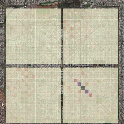
Aerial view of La Plata; a T-matrix; the two overlayed

Objective

This example illustrates the syntax to select specific multipole orders from each individual particle T-matrix. We also display the collective T-matrix of a cluster.

Unmasked matrices

We first start with a simulation using the following input file

where we run everything at a single wavelength to make it easier to display the different matrices.

The command to run the example is simply

../../build/terms input > log

The output consists of the standard far-field cross-sections in various files, with the addition of 3 files as requested:

prestagedA.txt (hard-coded name, single wavelength)
stagedA_bal.txt (hard-coded name, single wavelength)
collective_tmat.txt (user-defined name, can contain multiple wavelengths)

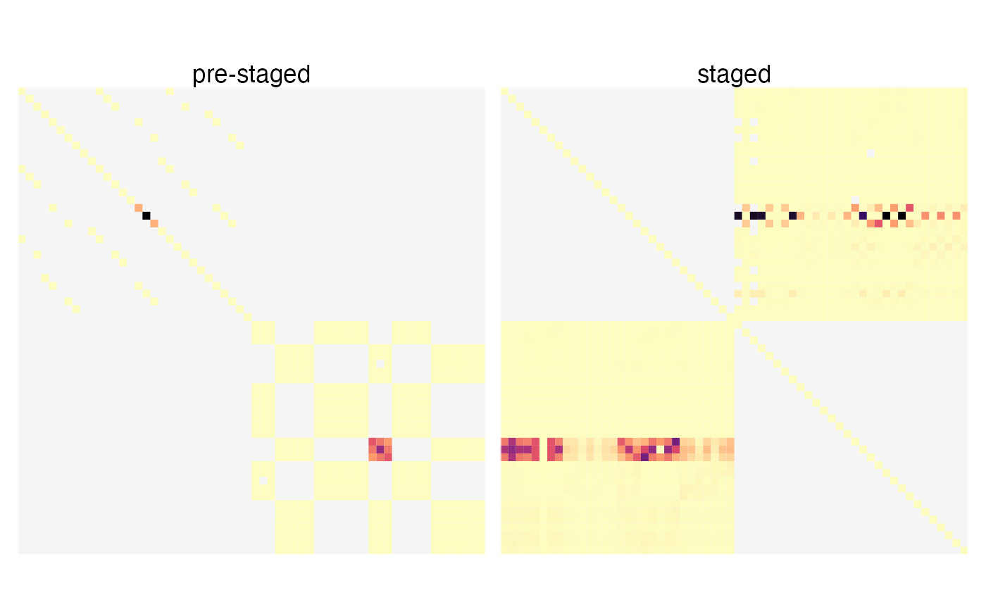
The “prestaged” matrix combines together the individual T-matrices for each scatterer, along the block-diagonal. Here we recognise that each particle’s T-matrix is dominated at this wavelength by the electric dipole resonance in the block \(T_{22}\). The first spheroid stays aligned with the lab frame, and is therefore diagonal, while the second particle, being rotated, mixes the different m values of the electric dipole.

The “staged” matrix presents the translation matrices involved in the off-diagonal blocks of the collective linear system solved by TERMS.

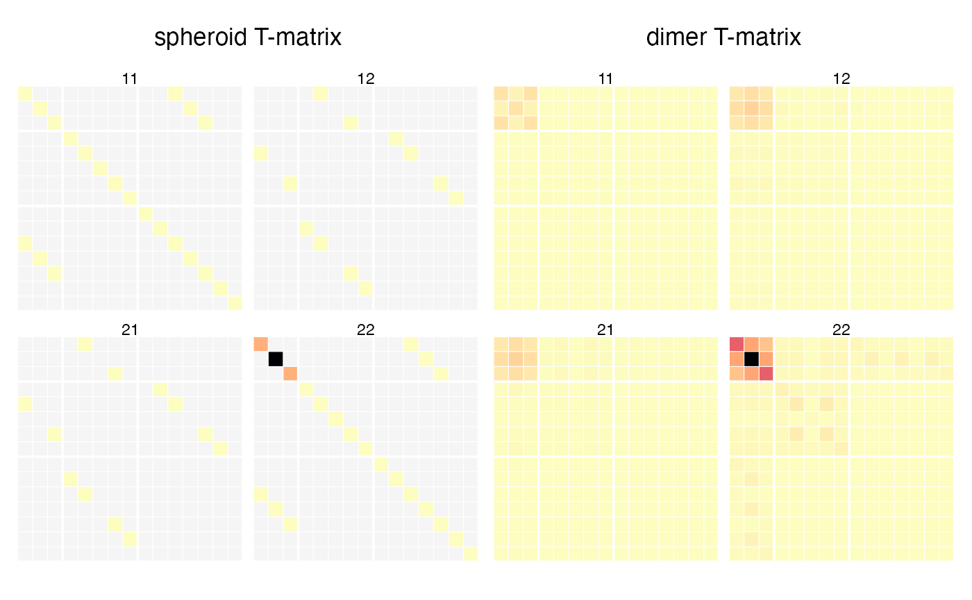
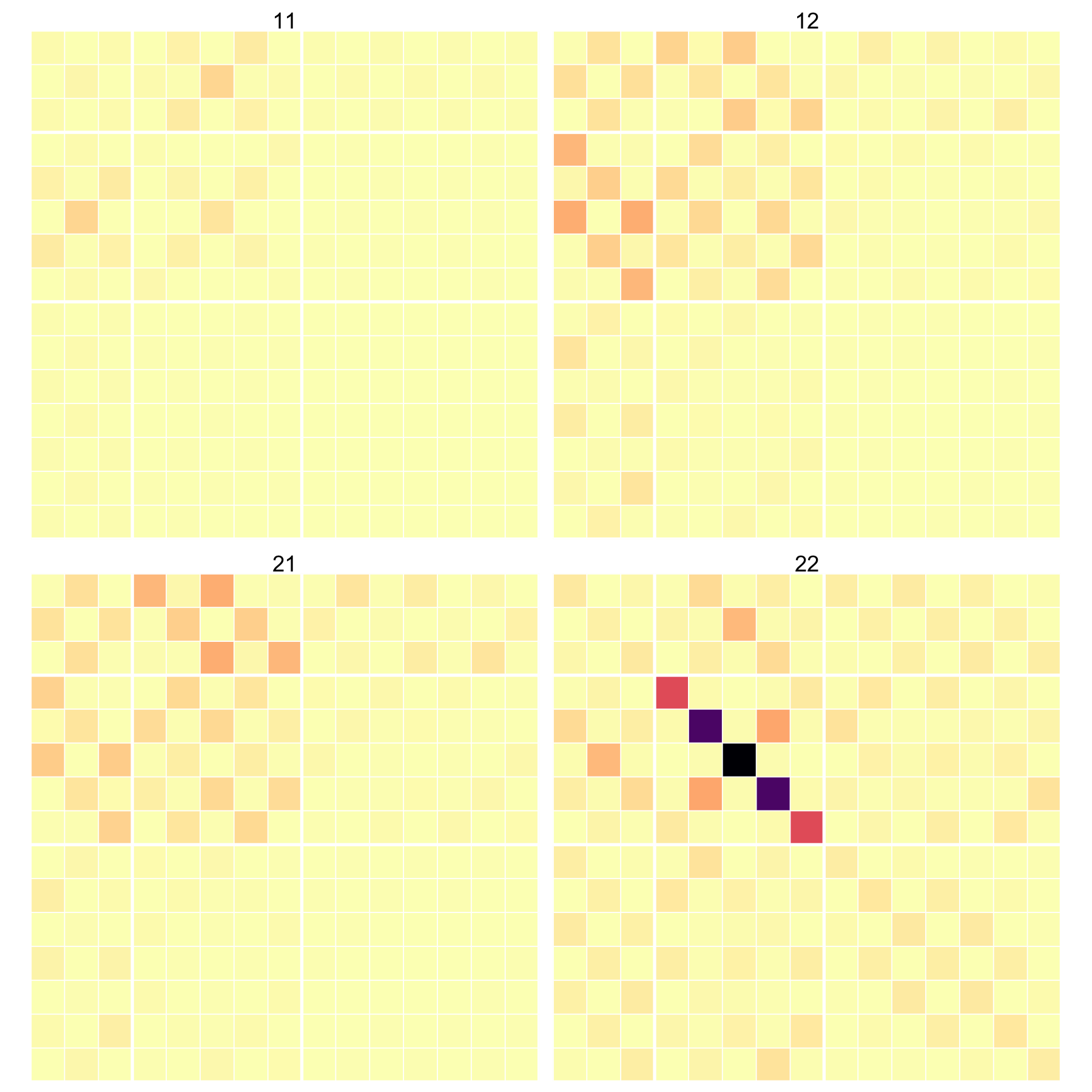
Once TERMS has solved the multiple scattering problem, it can export the collective T-matrix of the whole cluster. In contrast to the T-matrix of a single spheroid, the matrix is fully dense due to the interaction between the two particles.

Masked matrices

With this default situation in mind, we now turn to the ability to select specific multipoles in the input T-matrices. For instance, we’ll use the following input file to select only the electric dipole term, which was already dominant because of the plasmon resonance.

ModeAndScheme 2 3

MultipoleCutoff 4
Medium 1.7689

OutputFormat HDF5 EE1

DumpPrestagedA
DumpStagedA
DumpCollectiveTmatrix collective_tmat_EE1.tmat

MultipoleSelections 1
EE1:1_MM2:1_ME2:1_EM2:1  blocks

Wavelength 650

Medium 1.7689

TmatrixFiles 1
"tmat_Au10x20_Nmax4_lambda650.tmat" 

# dimer, dihedral pi/4
Scatterers 2
TF1_S1 0 -50 0.0 50 0.0 0.0 0.0  2.5
TF1_S1 0  50 0.0 50 0.0 0.7853982 0  2.5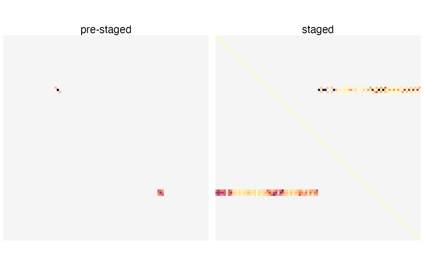

As a last example we now select the electric quadrupole, and mask all other orders,

ModeAndScheme 2 3

MultipoleCutoff 4

OutputFormat HDF5 EE2_MM0

DumpPrestagedA
DumpStagedA
DumpCollectiveTmatrix collective_tmat_EE2_MM0.tmat

MultipoleSelections 1
EE2:2_MM2:1_ME2:1_EM2:1  blocks

Wavelength 650

Medium 1.7689

TmatrixFiles 1
"tmat_Au10x20_Nmax4_lambda650.tmat" 

# dimer, dihedral pi/4
Scatterers 2
TF1_S1 0 -50 0.0 50 0.0 0.0 0.0  2.5
TF1_S1 0  50 0.0 50 0.0 0.7853982 0  2.5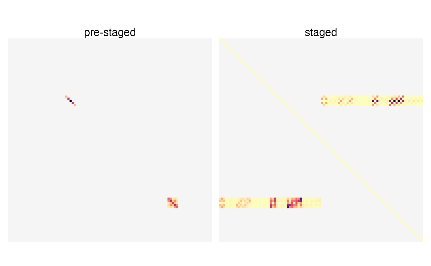

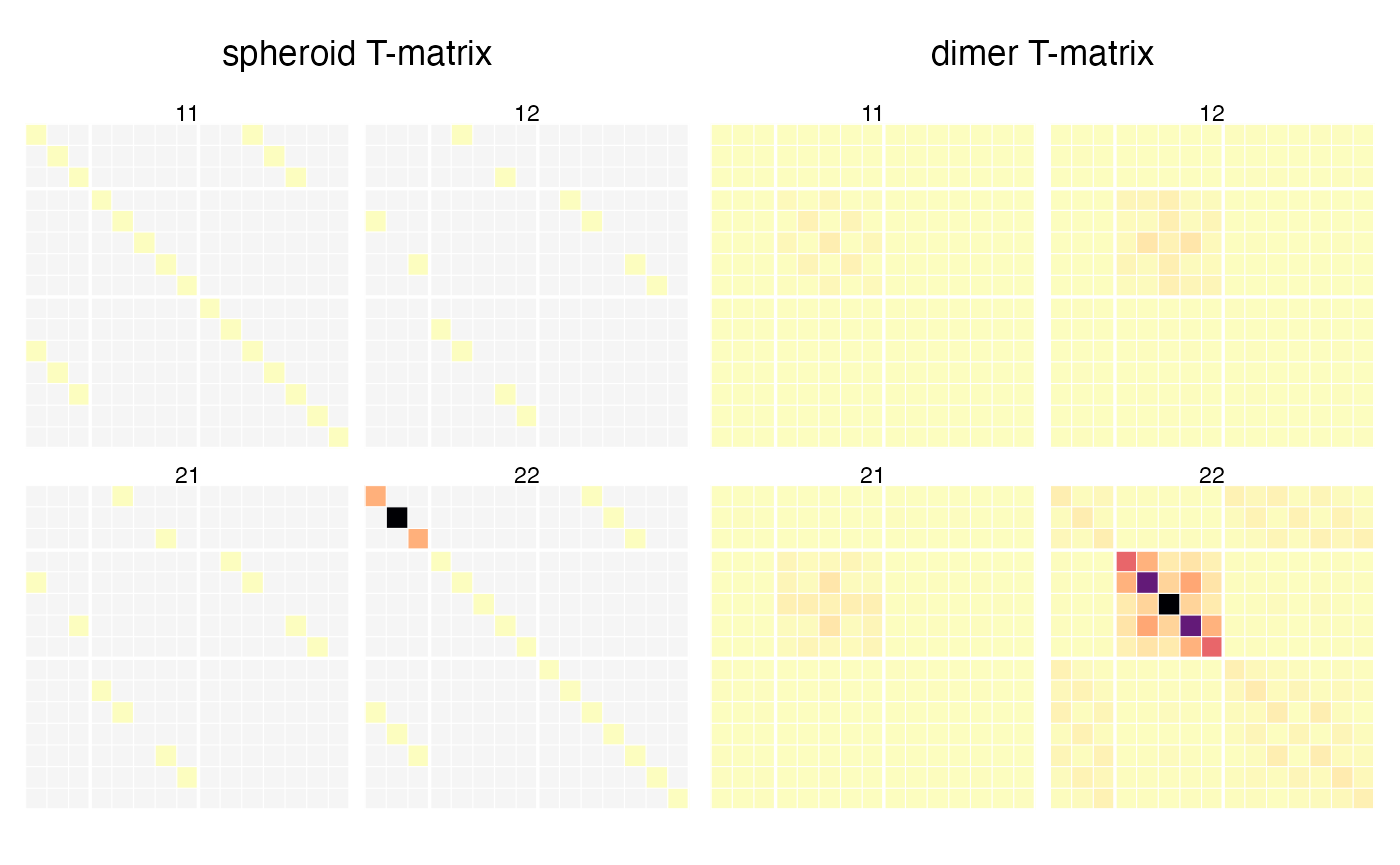
With these input T-matrices being masked without the strong electric dipole component, the collective T-matrix is now very different.

Last run: 05 December, 2023