Polarised orientation-averaged local field intensities
05 December, 2023
Source:vignettes/111_polarised_nf/111_polarised_nf.Rmd
111_polarised_nf.RmdObjective
This example illustrates the calculation of orientation-averaged
local field intensities for separate circular polarisations, using the
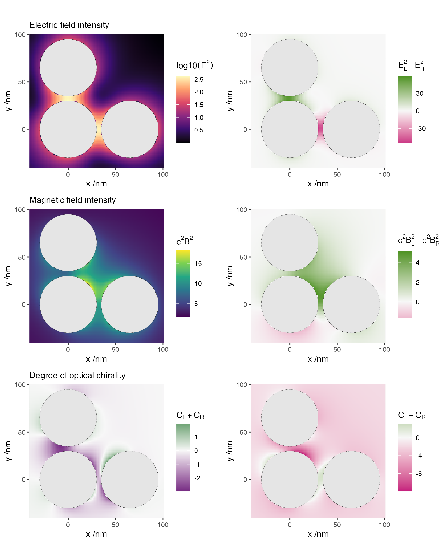
keyword MapOaQuantity [p]. The structure consists of a
tetramer of Au spheres. Because the structure is chiral, the local
fields depend on the handedness of the incident light, even after full
orientation averaging.
-
MapOaQuantity unpolarised: returns orientation-averaged near fields, also averaged over polarisation -
MapOaQuantity polarised, withIncidence 0 0 0 1triggering both L and R polarisations -
MapOaQuantity polarised, withIncidence 0 0 0 2triggering only R polarisation
ModeAndScheme 1 2
Wavelength 600
MultipoleCutoff 3
Medium 1.7689

OutputFormat HDF5 map_L

SpacePoints -40 100 100 -40 100 100 0 0 0 0 0 0
MapOaQuantity polarised
Incidence 0 0 0 -2 # L only

Scatterers 4
Au 0 65 0 30
Au 0 0 0 30
Au 65 0 0 30
Au 65 0 65 30
For a given (L) polarisation we obtain:
Rows: 10,201
Columns: 7
$ wavelength <dbl> 600, 600, 600, 600, 600, 600, 600, 600, 600, 600, 600, 600,…
$ x          <dbl> -40, -40, -40, -40, -40, -40, -40, -40, -40, -40, -40, -40,…
$ y          <dbl> -40.0, -38.6, -37.2, -35.8, -34.4, -33.0, -31.6, -30.2, -28…
$ z          <dbl> 0, 0, 0, 0, 0, 0, 0, 0, 0, 0, 0, 0, 0, 0, 0, 0, 0, 0, 0, 0,…
$ `E^2`      <dbl> 2.598977, 2.732408, 2.875605, 3.029059, 3.193237, 3.368563,…
$ `B^2`      <dbl> 2.591401e-17, 2.617457e-17, 2.644542e-17, 2.672731e-17, 2.7…
$ `C^2`      <dbl> 1.067857, 1.078401, 1.089044, 1.099723, 1.110363, 1.120874,…
For unpolarised incidence:
Rows: 10,201
Columns: 6
$ wavelength <dbl> 600, 600, 600, 600, 600, 600, 600, 600, 600, 600, 600, 600,…
$ x          <dbl> -40, -40, -40, -40, -40, -40, -40, -40, -40, -40, -40, -40,…
$ y          <dbl> -40.0, -38.6, -37.2, -35.8, -34.4, -33.0, -31.6, -30.2, -28…
$ z          <dbl> 0, 0, 0, 0, 0, 0, 0, 0, 0, 0, 0, 0, 0, 0, 0, 0, 0, 0, 0, 0,…
$ `E^2`      <dbl> 2.659462, 2.795008, 2.940230, 3.095586, 3.261501, 3.438356,…
$ `B^2`      <dbl> 2.481858e-17, 2.505532e-17, 2.530400e-17, 2.556574e-17, 2.5…
For both polarisations:
Rows: 10,201
Columns: 10
$ wavelength <dbl> 600, 600, 600, 600, 600, 600, 600, 600, 600, 600, 600, 600,…
$ x          <dbl> -40, -40, -40, -40, -40, -40, -40, -40, -40, -40, -40, -40,…
$ y          <dbl> -40.0, -38.6, -37.2, -35.8, -34.4, -33.0, -31.6, -30.2, -28…
$ z          <dbl> 0, 0, 0, 0, 0, 0, 0, 0, 0, 0, 0, 0, 0, 0, 0, 0, 0, 0, 0, 0,…
$ `E^2[L]`   <dbl> 2.719948, 2.857607, 3.004855, 3.162113, 3.329765, 3.508150,…
$ `E^2[R]`   <dbl> 2.598977, 2.732408, 2.875605, 3.029059, 3.193237, 3.368563,…
$ `B^2[L]`   <dbl> 2.372315e-17, 2.393606e-17, 2.416259e-17, 2.440417e-17, 2.4…
$ `B^2[R]`   <dbl> 2.591401e-17, 2.617457e-17, 2.644542e-17, 2.672731e-17, 2.7…
$ `C[L]`     <dbl> -1.0028411, -1.0100127, -1.0171346, -1.0241537, -1.0310116,…
$ `C[R]`     <dbl> 1.067857, 1.078401, 1.089044, 1.099723, 1.110363, 1.120874,…
Maps
We now map the orientation-averaged local electric and magnetic field intensity and local degree of optical chirality (LDOC) in the z=0 plane, for unpolarised excitation, and the difference between L and R polarisations. Note that only the unpolarised electric field intensity is displayed in log scale. The calculations inside the spheres are not reliable and therefore not displayed.
For unpolarised LDOC, we simply average the two polarisations, as no formula is readily available.
Last run: 05 December, 2023