Angular dispersion
05 December, 2023
Source:vignettes/02_angular_dispersion/02_angular_dispersion.Rmd
02_angular_dispersion.RmdObjective
This example illustrates the calculation of far-field cross-sections for multiple angles of incidence. The structure consists of two silver spheres in water, and all parameters are kept to their default values.
This simulation uses the following input file
ModeAndScheme 2 3
MultipoleCutoff 5
Wavelength 300 700 200
Medium 1.7689 # epsilon of water
OutputFormat HDF5 results

Incidence  -7 0.0 0.0 4 1 1 # 7 incidences along phi in [0, pi/2]

Scatterers 2
Ag -40.0 0.0 0.0 30.0
Ag  40.0 0.0 0.0 30.0
The command to run the example is simply
../../build/terms input > logThe full log contains basic details of the calculations, and finishes with the timing.
Show log file (click to open)
readInputFile> Parsing file input

readInputFile> Detected keyword ModeAndScheme
               mode=2 => spectrum_FF for far-field quantities
               scheme=3 => Seek T^(j) using Mackowski's approach
readInputFile> Detected keyword MultipoleCutoff
               Supplied ncut(1)=  5
               Setting ncut(2)= ncut(1)
               Setting ncut(3)=  -8
readInputFile> Detected keyword Wavelength
               Wavelength LB (nm):   300.000000
               Wavelength UB (nm):   700.000000
               nsteps, step:       200    2.0000
readInputFile> Detected keyword Medium
               Constant host epsilon=  1.7689E+0
readInputFile> Detected keyword OutputFormat
               OutputFormat=HDF5
               All output files are stored in file "results.h5                                                      "
readInputFile> Detected keyword Incidence
readInputFile> Euler angle alpha [0,2Pi) grid-points:    7
readInputFile> Modified alpha maximum:   1.57079633
readInputFile> Euler angle beta  [0,Pi]  value=   0.00000000
readInputFile> Euler angle gamma [0,2Pi) value=   0.00000000
               Incident Euler angles and weights:
                  alpha        beta        gamma        weight
               0.11219974   0.00000000   0.00000000   0.14285714
               0.33659921   0.00000000   0.00000000   0.14285714
               0.56099869   0.00000000   0.00000000   0.14285714
               0.78539816   0.00000000   0.00000000   0.14285714
               1.00979764   0.00000000   0.00000000   0.14285714
               1.23419711   0.00000000   0.00000000   0.14285714
               1.45859659   0.00000000   0.00000000   0.14285714

readInputFile> Detected keyword Scatterers
 with nscat=    2

readInputFile> Descriptor(s) and circumscribing sphere(s):

 scatID String                  x          y          z         R_0
    1   Ag                 -4.0000E+1  0.0000E+0  0.0000E+0  3.0000E+1
    2   Ag                  4.0000E+1  0.0000E+0  0.0000E+0  3.0000E+1

readInputFile> Individual geometry characteristic(s):

 scatID Details
    1   Mie with ncoats= 0
    2   Mie with ncoats= 0

readInputFile> Dielectric functions for (coated) Mie scatterer(s):

 scatID volID Label
    1     0     Ag
    2     0     Ag

readInputFile> Finished parsing  7 keywords


spectrumFF> ===== Wavelength:   300.00 (nm) ======================

solve> Prestaging...
solve> Staging and solving/inverting...
solve> Done!
...
termsProgram> Program run time (CPU & real in s):  1.534E+00  1.348E+00
The output consists of a single hdf5 file, storing the far-field cross-sections for each order from 1 to \(n_{1}\) for orientation-averaged quantities (as in example 01), and for each angle of incidence for fixed-orientation quantities, preceded by their average,
Show file results.h5 (click to open)
                           group                 name       otype dclass
0                              /            Far-Field   H5I_GROUP
1                     /Far-Field           Incidences H5I_DATASET  FLOAT
2                     /Far-Field          Wavelengths H5I_DATASET  FLOAT
3                     /Far-Field      fixed_incidence   H5I_GROUP
4     /Far-Field/fixed_incidence              csAbs1X H5I_DATASET  FLOAT
5     /Far-Field/fixed_incidence              csAbs2Y H5I_DATASET  FLOAT
6     /Far-Field/fixed_incidence              csAbs3R H5I_DATASET  FLOAT
7     /Far-Field/fixed_incidence              csAbs4L H5I_DATASET  FLOAT
8     /Far-Field/fixed_incidence              csExt1X H5I_DATASET  FLOAT
9     /Far-Field/fixed_incidence              csExt2Y H5I_DATASET  FLOAT
10    /Far-Field/fixed_incidence              csExt3R H5I_DATASET  FLOAT
11    /Far-Field/fixed_incidence              csExt4L H5I_DATASET  FLOAT
12    /Far-Field/fixed_incidence              csSca1X H5I_DATASET  FLOAT
13    /Far-Field/fixed_incidence              csSca2Y H5I_DATASET  FLOAT
14    /Far-Field/fixed_incidence              csSca3R H5I_DATASET  FLOAT
15    /Far-Field/fixed_incidence              csSca4L H5I_DATASET  FLOAT
16                    /Far-Field         oa_incidence   H5I_GROUP
17       /Far-Field/oa_incidence              cdAbsOA H5I_DATASET  FLOAT
18       /Far-Field/oa_incidence              cdExtOA H5I_DATASET  FLOAT
19       /Far-Field/oa_incidence              cdScaOA H5I_DATASET  FLOAT
20       /Far-Field/oa_incidence              csAbsOA H5I_DATASET  FLOAT
21       /Far-Field/oa_incidence              csExtOA H5I_DATASET  FLOAT
22       /Far-Field/oa_incidence              csScaOA H5I_DATASET  FLOAT
23                    /Far-Field   partial_absorption   H5I_GROUP
24 /Far-Field/partial_absorption csAbs1X_scat001coat0 H5I_DATASET  FLOAT
25 /Far-Field/partial_absorption csAbs1X_scat002coat0 H5I_DATASET  FLOAT
26 /Far-Field/partial_absorption csAbs2Y_scat001coat0 H5I_DATASET  FLOAT
27 /Far-Field/partial_absorption csAbs2Y_scat002coat0 H5I_DATASET  FLOAT
28 /Far-Field/partial_absorption csAbs3R_scat001coat0 H5I_DATASET  FLOAT
29 /Far-Field/partial_absorption csAbs3R_scat002coat0 H5I_DATASET  FLOAT
30 /Far-Field/partial_absorption csAbs4L_scat001coat0 H5I_DATASET  FLOAT
31 /Far-Field/partial_absorption csAbs4L_scat002coat0 H5I_DATASET  FLOAT
       dim
0
1    7 x 4
2      201
3
4  201 x 8
5  201 x 8
6  201 x 8
7  201 x 8
8  201 x 8
9  201 x 8
10 201 x 8
11 201 x 8
12 201 x 8
13 201 x 8
14 201 x 8
15 201 x 8
16
17 201 x 6
18 201 x 6
19 201 x 6
20 201 x 6
21 201 x 6
22 201 x 6
23
24 201 x 8
25 201 x 8
26 201 x 8
27 201 x 8
28 201 x 8
29 201 x 8
30 201 x 8
31 201 x 8
List of 3
$ mCOA: tibble [3,618 × 5] (S3: tbl_df/tbl/data.frame)
..$ wavelength: num [1:3618] 300 300 300 300 300 300 302 302 302 302 ...
..$ crosstype : chr [1:3618] "Abs" "Abs" "Abs" "Abs" ...
..$ variable : chr [1:3618] "total" "I1" "I2" "I3" ...
..$ dichroism : num [1:3618] 5.40e-13 2.25e-13 1.40e-14 2.88e-13 1.26e-14 ...
..$ average : num [1:3618] 504.4 367.13 117.67 18.2 1.34 ...
$ mCFO: tibble [4,824 × 7] (S3: tbl_df/tbl/data.frame)
..$ wavelength : num [1:4824] 300 300 300 300 300 300 300 300 302 302 ...
..$ crosstype : chr [1:4824] "Abs" "Abs" "Abs" "Abs" ...
..$ variable : chr [1:4824] "total" "I1" "I2" "I3" ...
..$ polarisation1: num [1:4824] 517 517 517 517 517 ...
..$ polarisation2: num [1:4824] 517 517 517 517 517 ...
..$ dichroism : num [1:4824] -1.07e-11 -1.36e-11 -1.00e-11 -1.14e-11 -1.14e-11 ...
..$ average : num [1:4824] 517 517 517 517 517 ...
$ mLFO: tibble [4,824 × 7] (S3: tbl_df/tbl/data.frame)
..$ wavelength : num [1:4824] 300 300 300 300 300 300 300 300 302 302 ...
..$ crosstype : chr [1:4824] "Abs" "Abs" "Abs" "Abs" ...
..$ variable : chr [1:4824] "total" "I1" "I2" "I3" ...
..$ polarisation1: num [1:4824] 517 441 456 483 517 ...
..$ polarisation2: num [1:4824] 517 593 578 551 517 ...
..$ dichroism : num [1:4824] -2.50e-12 -1.52e+02 -1.22e+02 -6.77e+01 -3.18e-12 ...
..$ average : num [1:4824] 517 517 517 517 517 ...Fixed-orientation results
The following files contain fixed-orientation cross-sections for X and Y linear polarisations,
Rows: 4,824
Columns: 7
$ wavelength    <dbl> 300, 300, 300, 300, 300, 300, 300, 300, 302, 302, 302, 3…
$ crosstype     <chr> "Abs", "Abs", "Abs", "Abs", "Abs", "Abs", "Abs", "Abs", …
$ variable      <chr> "total", "I1", "I2", "I3", "I4", "I5", "I6", "I7", "tota…
$ polarisation1 <dbl> 516.7623, 440.6962, 455.7620, 482.9097, 516.7623, 550.61…
$ polarisation2 <dbl> 516.7623, 592.8283, 577.7625, 550.6148, 516.7623, 482.90…
$ dichroism     <dbl> -2.501110e-12, -1.521321e+02, -1.220005e+02, -6.770514e+…
$ average       <dbl> 516.7623, 516.7623, 516.7623, 516.7623, 516.7623, 516.76…
tibble [8,442 × 7] (S3: tbl_df/tbl/data.frame)
$ wavelength: num [1:8442] 300 300 300 300 300 300 300 300 300 300 ...
$ crosstype : chr [1:8442] "Abs" "Abs" "Abs" "Abs" ...
$ variable : chr [1:8442] "I1" "I1" "I2" "I2" ...
$ dichroism : num [1:8442] -152.1 -152.1 -122 -122 -67.7 ...
$ average : num [1:8442] 517 517 517 517 517 ...
$ name : chr [1:8442] "polarisation1" "polarisation2" "polarisation1" "polarisation2" ...
$ value : num [1:8442] 441 593 456 578 483 ...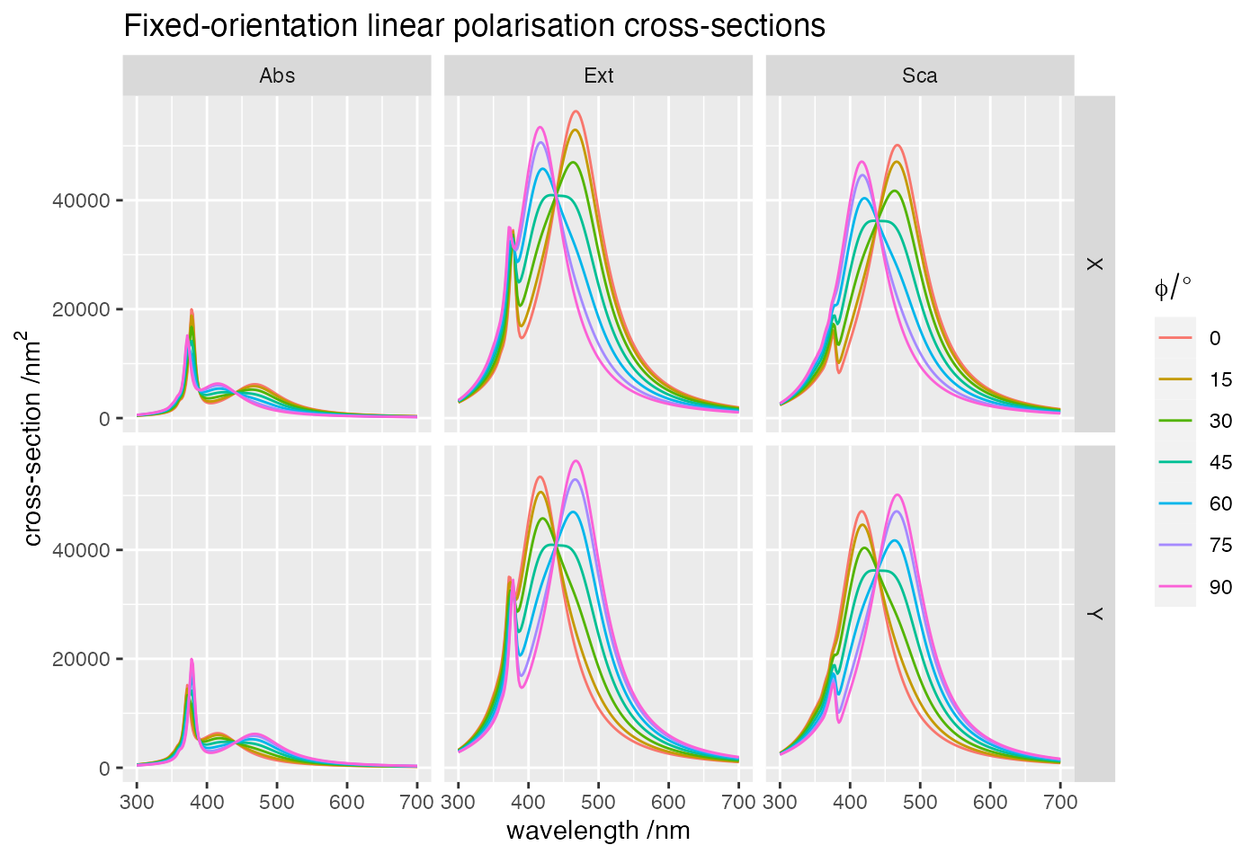
Because we are rotating \(\phi\) from 0 to 90 degrees, the two polarisations show the opposite trend as the incident electric field rotates from x to y.
Last run: 05 December, 2023