Objective
This example considers the scaling of computational time with respect to key parameters:
- number of particles
- number of multipoles
- number of incidence angles
- solution scheme
The number of wavelengths simply scales the computation time for all other parameters, as everything needs to be re-calculated for each wavelength (assuming negligible input-output time, compared to the calculations).
Parameters
The structure consists of a helix of gold spheres, with varying number of particles.
ModeAndScheme 2 {scheme}
MultipoleCutoff {Nmax}
{comment_centred}ScattererCentredCrossSections
Incidence {Ninc} 0.0 0.0 1
OutputFormat HDF5 xsec_{Npart}_{Ninc}_{Nmax}_{comment_centred}
Wavelength 633
Medium 1.7689 # epsilon of water
Verbosity 3 # show timings

Scatterers  {Npart}
The timings are collected from the log files, and stored with the corresponding subroutine name (and detail where applicable),
Rows: 53,722
Columns: 10
$ Npart   <dbl> 1, 1, 1, 1, 1, 1, 1, 1, 1, 1, 1, 1, 1, 1, 1, 1, 1, 1, 1, 1, 1,…
$ Nmax    <dbl> 8, 8, 8, 8, 8, 8, 8, 8, 8, 8, 8, 8, 8, 8, 8, 8, 8, 8, 8, 8, 8,…
$ Ninc    <dbl> 1, 1, 1, 1, 1, 1, 1, 1, 1, 1, 1, 1, 1, 1, 1, 1, 1, 1, 1, 1, 1,…
$ scheme  <int> 0, 0, 0, 0, 0, 0, 0, 0, 0, 0, 0, 0, 0, 0, 0, 0, 0, 0, 0, 0, 1,…
$ centred <dbl> 1, 1, 1, 1, 1, 1, 1, 1, 1, 1, 1, 1, 1, 1, 1, 1, 1, 1, 1, 1, 1,…
$ log     <chr> "1", "1", "1", "1", "1", "1", "1", "1", "1", "1", "1", "1", "1…
$ routine <chr> "solve", "solve", "solve", "solve", "solve", "solve", "solve",…
$ detail  <chr> "calcSphBessels (reg. & irreg)", "calcMieTMat", "calcWignerBig…
$ cpu     <dbl> 0.001346, 0.003255, 0.000000, 0.013800, 0.000703, 0.104900, 0.…
$ total   <dbl> 0.000, 0.000, 0.000, 0.001, 0.000, 0.009, 0.000, 0.000, 0.000,…
Total timings
We first look at the total run time summaries, as a function of number of particles \(Npart\), multipolar order \(Nmax\), and number of incidence directions \(Ninc\).

Detailed timings (subroutines)
At Verbosity > 0 we can also access the timings
within subroutines, to break down the calculation and identify
time-consuming steps.
tibble [53,722 × 10] (S3: tbl_df/tbl/data.frame)
 $ Npart  : num [1:53722] 1 1 1 1 1 1 1 1 1 1 ...
 $ Nmax   : num [1:53722] 8 8 8 8 8 8 8 8 8 8 ...
 $ Ninc   : num [1:53722] 1 1 1 1 1 1 1 1 1 1 ...
 $ scheme : int [1:53722] 0 0 0 0 0 0 0 0 0 0 ...
 $ centred: num [1:53722] 1 1 1 1 1 1 1 1 1 1 ...
 $ log    : chr [1:53722] "1" "1" "1" "1" ...
 $ routine: chr [1:53722] "solve" "solve" "solve" "solve" ...
 $ detail : chr [1:53722] "calcSphBessels (reg. & irreg)" "calcMieTMat" "calcWignerBigD" "stageAmat" ...
 $ cpu    : num [1:53722] 0.001346 0.003255 0 0.0138 0.000703 ...
 $ total  : num [1:53722] 0 0 0 0.001 0 0.009 0 0 0 0 ...
[1] "solve" "spectrumFF" "calcCsStout" "termsProgram" "contractTmat"
[6] "calcOaStout" "calcTIJStout"Some subroutines are broken down in more detail,
 [1] "calcSphBessels (reg. & irreg)"  "calcMieTMat"
 [3] "calcWignerBigD"                 "stageAmat"
 [5] "balanceVecJ"                    "solLinSys"
 [7] "invSqrMat"                      "balanceMatJI"
 [9] "calcTIJStout"                   "calcTIMackowski"
[11] "calcMieIntCoeffs"               "Solve: diff. incs"
[13] "calcVTACs"                      "calcCsStout"
[15] "partial abs. for Mie scatterer" NA
[17] "offsetTmat"                     "calcVTACsAxial"
[19] "contractTmat"                   "calcAbsMat"
[21] "calcOaStout"                    "calcOAprops"
[23] "post-inversion"
Varying number of particles
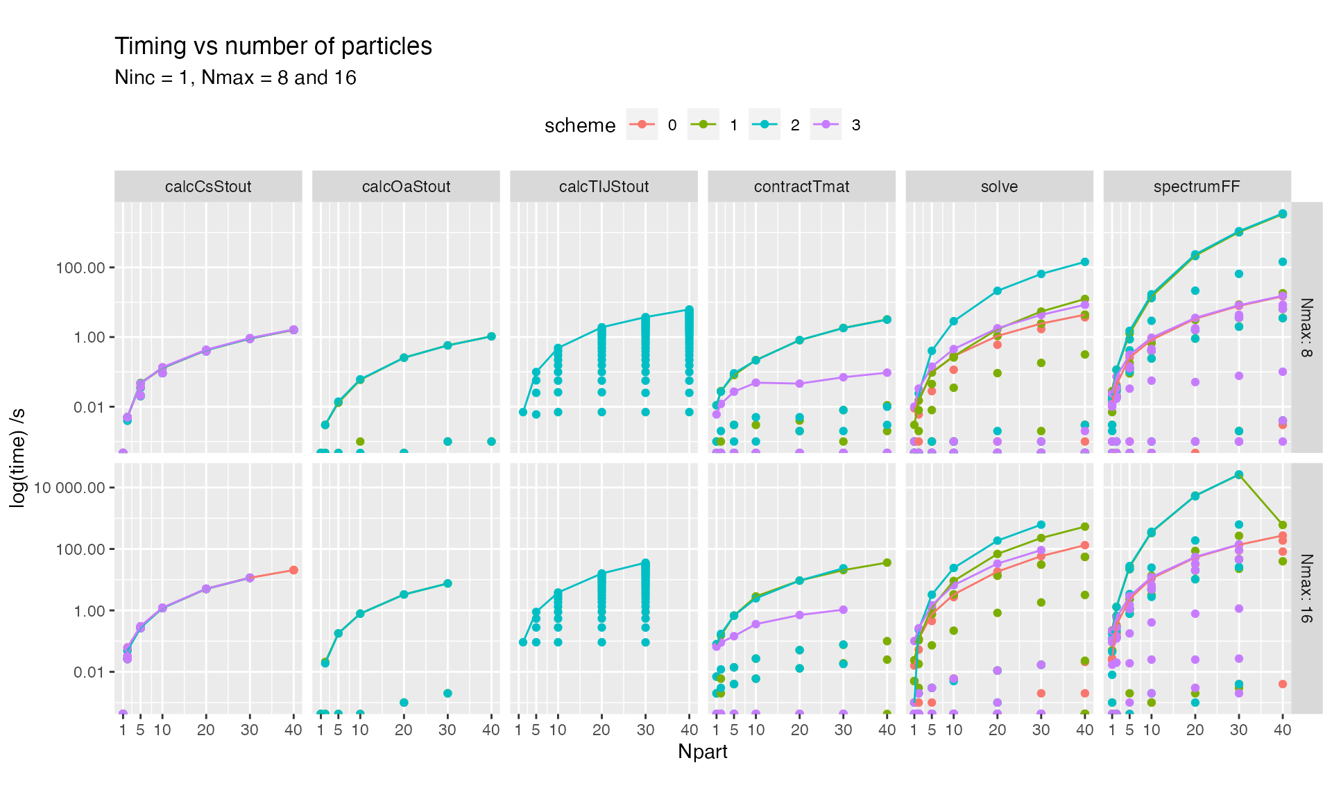
Details of the solve subroutine are shown below
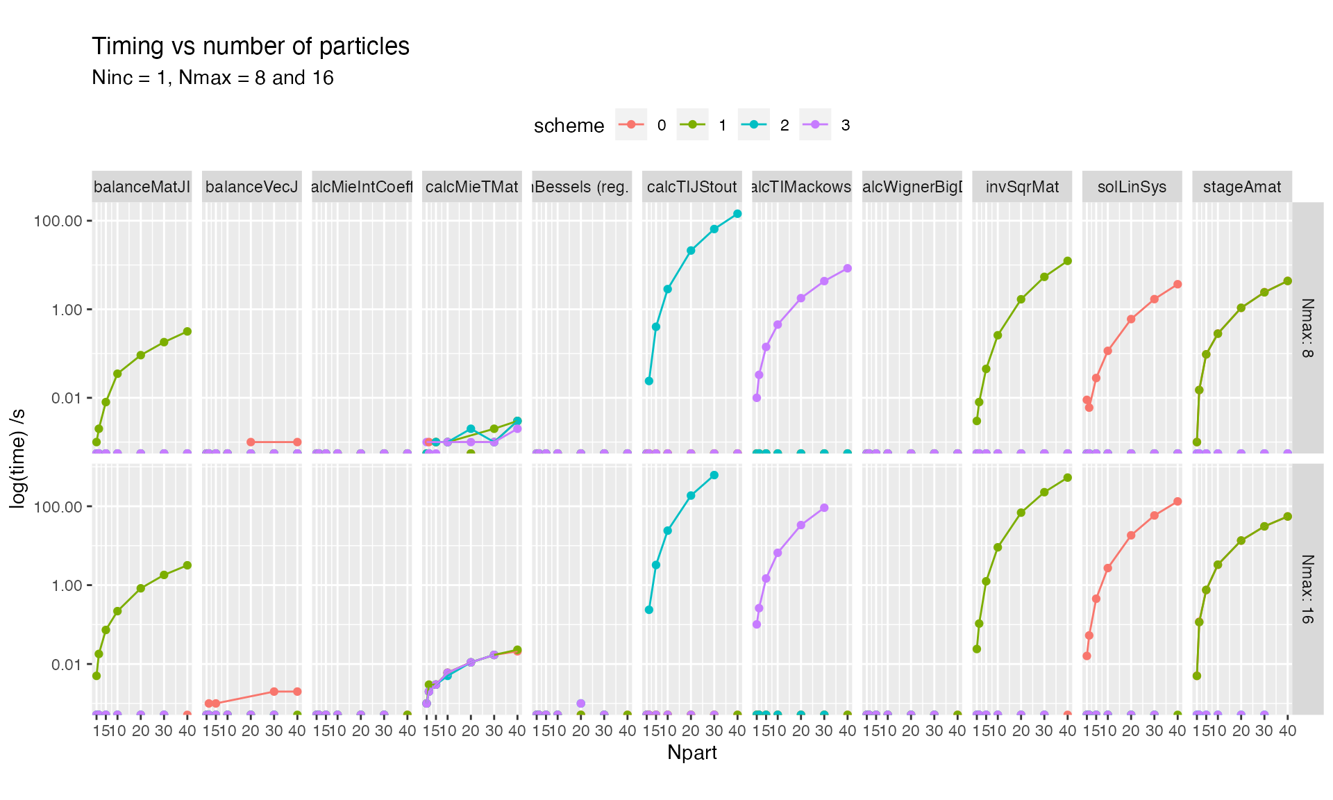
We can make some general remarks,
- The Stout Scheme (2) solves recursively the multiple scattering
problem, starting with a dimer, and adding one particle at a time. This
is evident in the routine
calcTIJStoutwhich increases in time. - Mackwoski’s Scheme (3) is very performant across the board; in fact it is about as fast as solving the original coupled-system without seeking the collective T-matrix, with the advantage that it also calculates orientation-averaged properties
Varying maximum multipole order
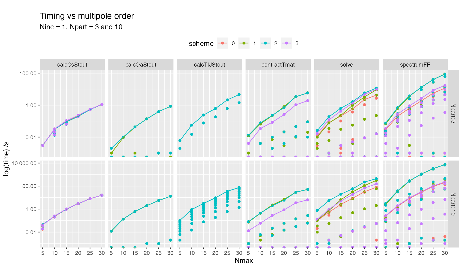
Details of the solve subroutine are shown below
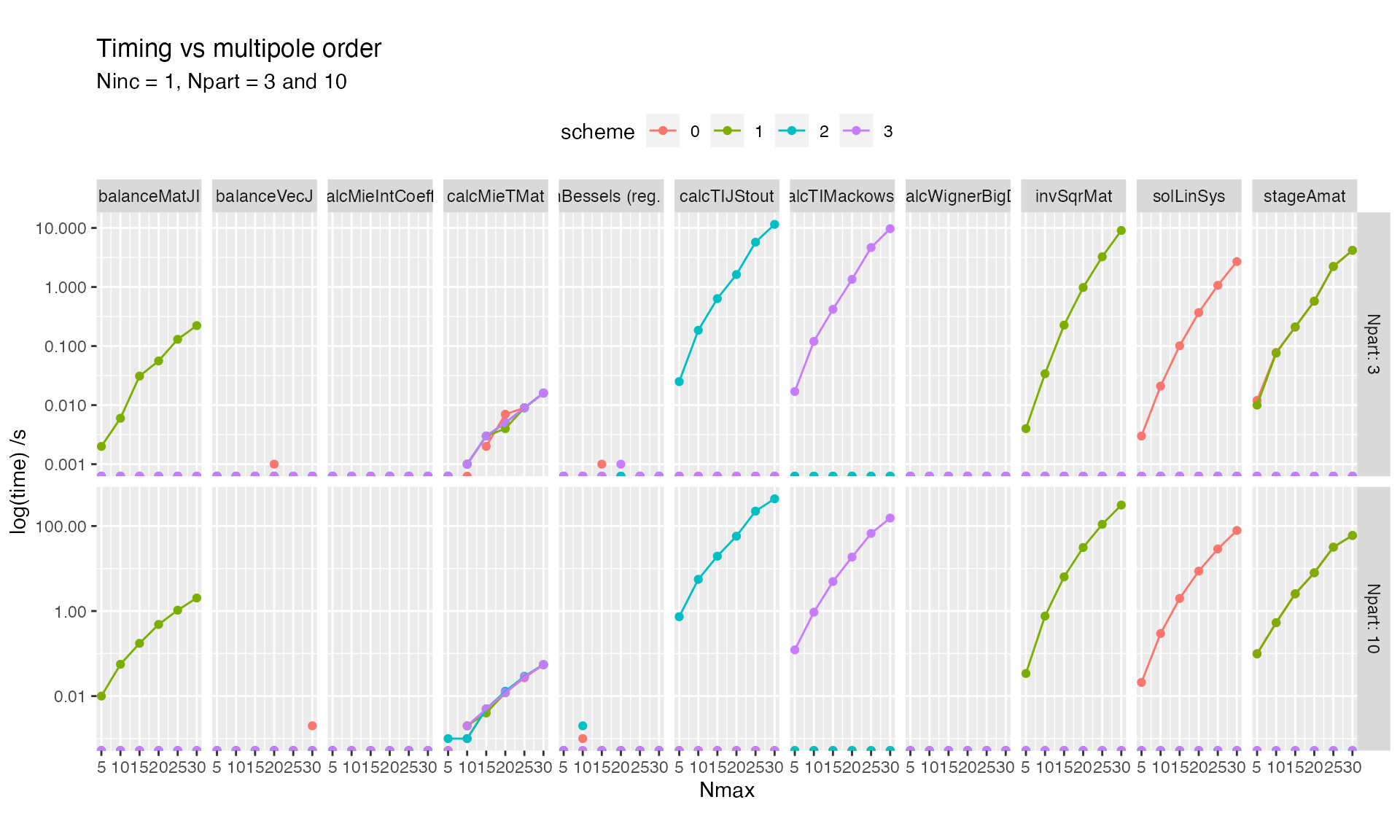
The computational cost scales similarly for all Schemes and subroutines with respect to maximum multipolar order.
Varying number of incidence directions
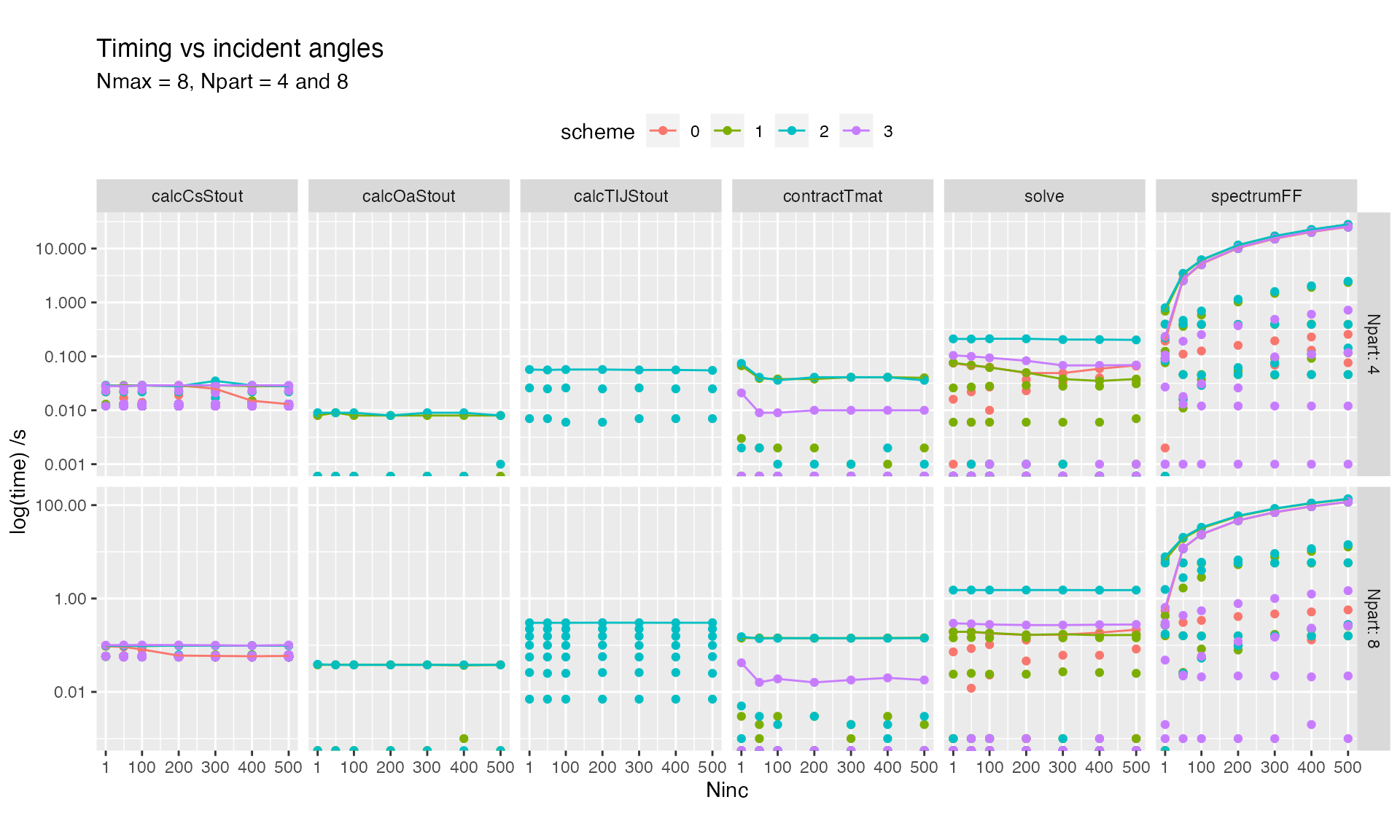
Details of the spectrumFF subroutine are shown below
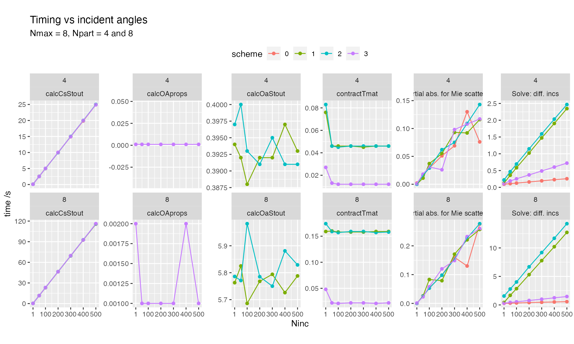
Details of the solve subroutine are shown below
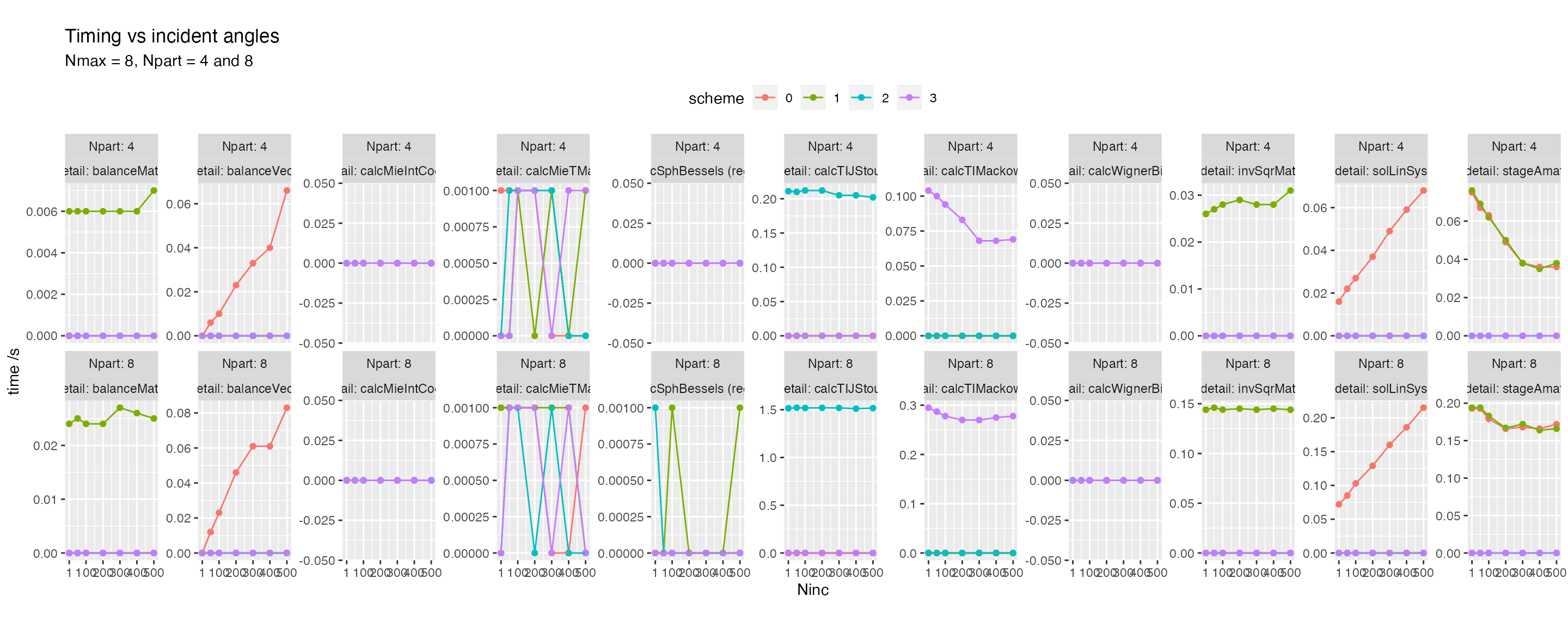
Solving a linear system for multiple incidences (right hand side)
differs between Scheme = 0 (direct solve) and the other
schemes (which seek a collective T-matrix). This is visible in routine
solLinSys, which shows linear scaling in
Scheme = 0 while Schemes 1, 2, 3 have almost constant
performance.
Curiously, the total timings rise sharply between 1 and 50 incidence angles for some schemes, suggesting that another subroutine is doing substantial computations. This may point to a possible optimisation in the future.
Last run: 05 December, 2023