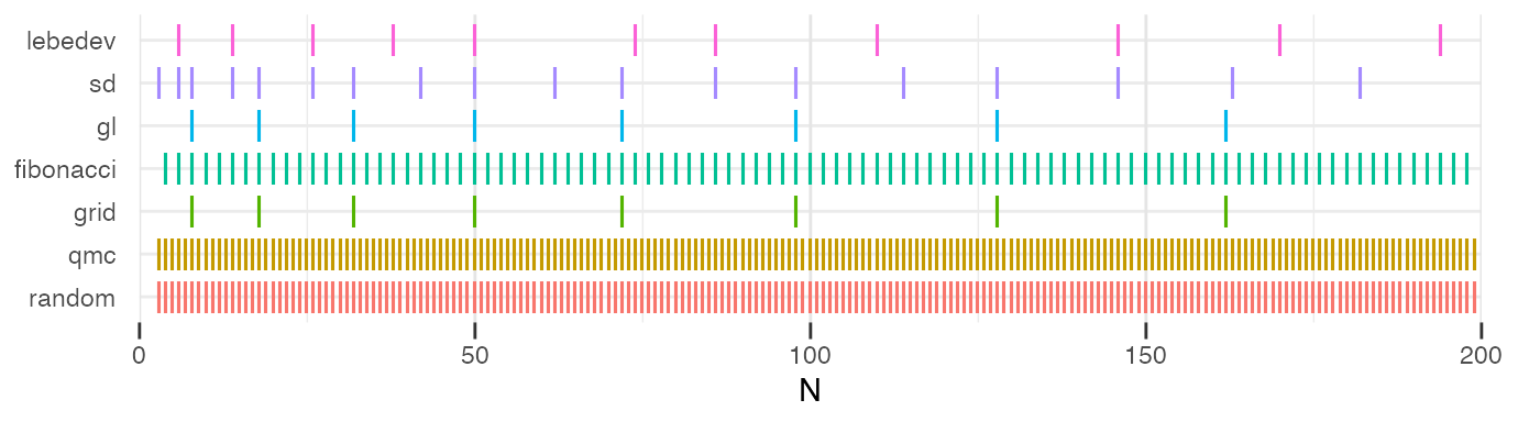
Overview of available cubatures
The main function of the package is cubs(N, method), where N is the requested number of integration points, and method one of the built-in cubature methods. The function returns a data.frame with three columns: phi, the azimuth (\(\varphi\in [0,2\pi]\)), theta, the polar angle (\(\theta\in [0,\pi]\)), and weight the associated cubature weight.
| phi | theta | weight |
|---|---|---|
| 0.000000 | 1.570796 | 0.1666667 |
| 3.141593 | 1.570796 | 0.1666667 |
| 1.570796 | 1.570796 | 0.1666667 |
| -1.570796 | 1.570796 | 0.1666667 |
| 1.570796 | 0.000000 | 0.1666667 |
| 1.570796 | 3.141593 | 0.1666667 |
| phi | theta | weight |
|---|---|---|
| 0.000000 | 0.000000 | 0.1666667 |
| 0.000000 | 1.570796 | 0.1666667 |
| -1.570796 | 1.570796 | 0.1666667 |
| 1.570796 | 1.570796 | 0.1666667 |
| 0.000000 | 3.141593 | 0.1666667 |
| 3.141593 | 1.570796 | 0.1666667 |
| phi | theta | weight |
|---|---|---|
| 0.000000 | 2.1862760 | 0.125 |
| 1.570796 | 2.1862760 | 0.125 |
| 3.141593 | 2.1862760 | 0.125 |
| 4.712389 | 2.1862760 | 0.125 |
| 0.000000 | 0.9553166 | 0.125 |
| 1.570796 | 0.9553166 | 0.125 |
| 3.141593 | 0.9553166 | 0.125 |
| 4.712389 | 0.9553166 | 0.125 |
| phi | theta | weight |
|---|---|---|
| 0.0000000 | 0.5856855 | 0.1666667 |
| 3.8832221 | 1.0471976 | 0.1666667 |
| 1.4832588 | 1.4033482 | 0.1666667 |
| 5.3664809 | 1.7382444 | 0.1666667 |
| 2.9665177 | 2.0943951 | 0.1666667 |
| 0.5665545 | 2.5559071 | 0.1666667 |
| phi | theta | weight |
|---|---|---|
| 0.7853982 | 2.094395 | 0.125 |
| 2.3561945 | 2.094395 | 0.125 |
| 3.9269908 | 2.094395 | 0.125 |
| 5.4977871 | 2.094395 | 0.125 |
| 0.7853982 | 1.047198 | 0.125 |
| 2.3561945 | 1.047198 | 0.125 |
| 3.9269908 | 1.047198 | 0.125 |
| 5.4977871 | 1.047198 | 0.125 |
| phi | theta | weight |
|---|---|---|
| 3.1415927 | 1.9106332 | 0.2 |
| 1.5707963 | 1.2309594 | 0.2 |
| 4.7123890 | 2.4619188 | 0.2 |
| 0.7853982 | 1.6821373 | 0.2 |
| 3.9269908 | 0.9817654 | 0.2 |
| phi | theta | weight |
|---|---|---|
| 5.2161769 | 1.2069112 | 0.2 |
| 1.5833269 | 2.3004085 | 0.2 |
| 3.7546088 | 0.7972976 | 0.2 |
| 4.2506012 | 0.8291747 | 0.2 |
| 0.1805071 | 0.9486489 | 0.2 |
Note that the requested number of points \(N\) is interpreted as a minimum number; the exact number of points will vary for each method, some having relatively sparse coverage.
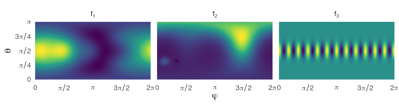
Test functions
We now compare the performance of these methods on 3 different integrands,
\[\begin{align} f_{1}(x, y, z)=& 1+x+y^{2}+x^{2} y + x^{4}+y^{5}+x^{2} y^{2} z^{2} \\ f_{2}(x, y, z)=& \tfrac{3}{4} e^{\left[-(9 x-2)^{2} / 4-(9 y-2)^{2} / 4-(9 z-2)^{2} / 4\right]} +\tfrac{3}{4} e^{\left[-(9 x+1)^{2} / 49-(9 y+1) / 10-(9 z+1) / 10\right]} +\tfrac{1}{2} e^{\left[-(9 x-7)^{2} / 4-(9 y-3)^{2} / 4-(9 z-5)^{2} / 4\right]}-\tfrac{1}{5} e^{\left[-(9 x-4)^{2}-(9 y-7)^{2}-(9 z-5)^{2}\right]} \\ f_{3}(\varphi, \theta)=& \tfrac{1}{4\pi} + \cos(12\varphi)\sin^{12}(\theta) \end{align}\] with the usual spherical coordinates, \[\begin{align} x = &\cos(\varphi)\sin(\theta)\\ y = & \sin(\varphi)\sin(\theta)\\ z = & \cos(\theta). \end{align}\]
Convergence comparison
We plot below the relative error against the known integrals (\(I_1 = 216\pi/35\), \(I_2 =6.6961822200736179523\dots\), \(I_3=1\)).
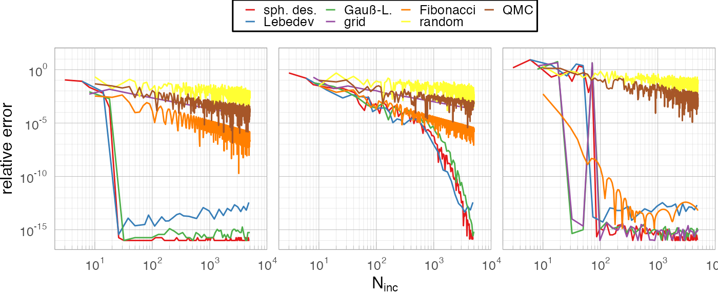
Three methods stand out and vastly outperform the others: Lebedev, Spherical t-Designs, and (somewhat behind) Gauß-Legendre. These cubature methods are known to integrate exactly spherical harmonics up to a given order, and are in that sense optimal choices (assuming the integrand is well-behaved in this basis).