The Kretschmann configuration is commonly used for sensing applications: the sharp resonance associated with the excitation of SPPs at the metal/dielectric interface is strongly sensitive about the refractive index of the dielectric medium. Furthermore, because SPPs are associated with a exponential decay of the electric field in the surrounding medium, the technique provides a surface-sensitive, sub-wavelength, probe.

Setting up

library(planar)
library(ggplot2)
require(reshape2)
library(gridExtra)
require(plyr)

We define a function to model our system with the parameters of interest: a semi-infinite incident medium (glass), a 50nm gold film, a thin layer of varying thickness and refractive index, and a semi-infinite dielectric medium of varying refractive index.

wvl <- 632.8
gold <- epsAu(wvl)
simulation <- function(thickness = 0, n1 = n2, n2 = 1) {
    results <- recursive_fresnelcpp(epsilon = list(1.5^2, gold$epsilon, n1^2, 
        n2^2), wavelength = gold$wavelength, thickness = c(0, 50, thickness, 
        0), angle = seq(0, pi/2, length = 2000), polarisation = "p")
    data.frame(results[c("angle", "R")])
}

Variation of the bulk medium

## loop over parameters
parameters <- function(res = 10) data.frame(n2 = seq(1, 1.5, length = res))

d1 <- mdply(parameters(10), simulation)
d2 <- mdply(parameters(300), simulation)

p1 <- ggplot(d1) + geom_line(aes(angle * 180/pi, R, colour = n2, group = n2)) + 
    scale_y_continuous("Reflectivity", expand = c(0, 0), limits = c(0, 1)) + 
    scale_x_continuous("Internal angle /degrees", expand = c(0, 0), breaks = seq(0, 
        90, by = 15)) + guides(colour = guide_legend())

## colour map
p2 <- ggplot(d2) + geom_raster(aes(angle * 180/pi, n2, fill = R)) + scale_y_continuous("n", 
    expand = c(0, 0)) + scale_x_continuous("Internal angle /degrees", expand = c(0, 
    0), breaks = seq(0, 90, by = 15))

grid.arrange(p1, p2, nrow = 1)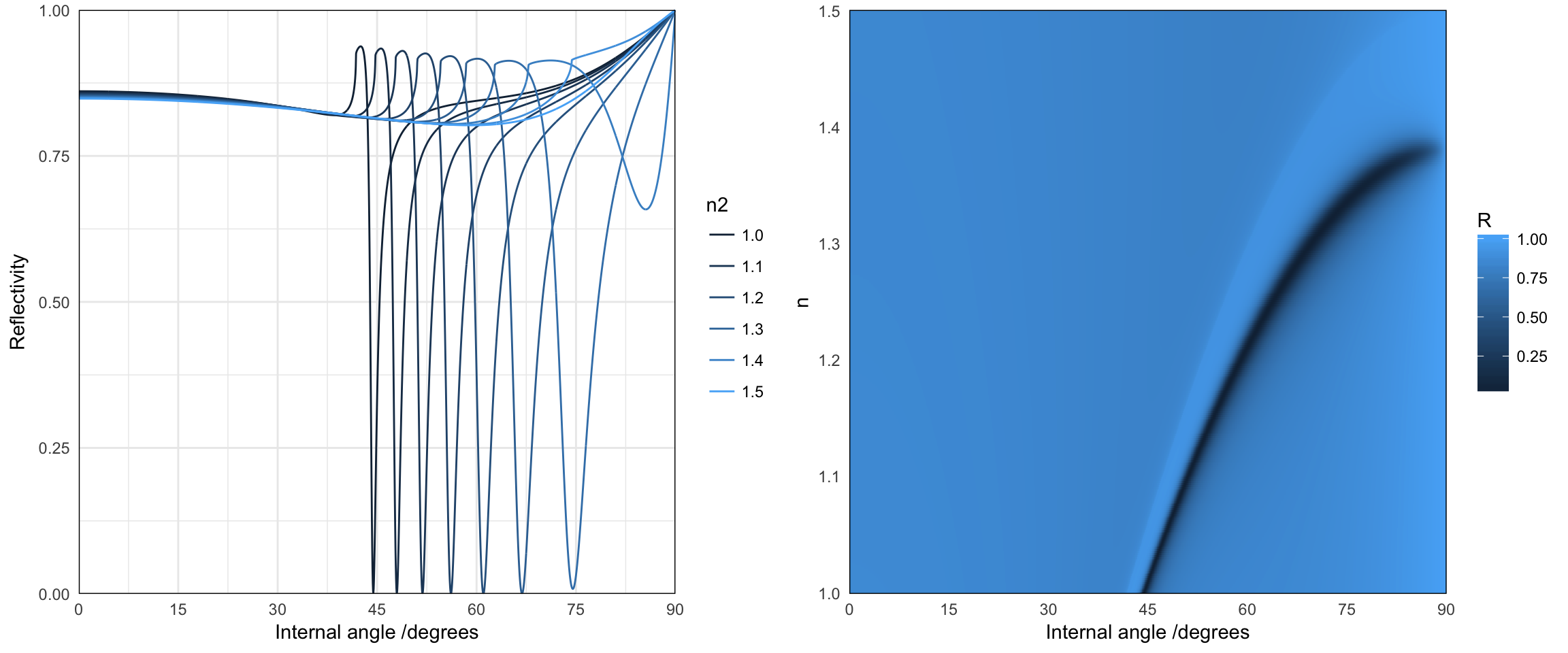

Local sensitivity

We now look at the effect of changing the refractive index of a thin layer, of varying thickness.

## loop over parameters
parameters <- function(res = 10) expand.grid(thickness = c(10, 50, 100, 400), 
    n1 = seq(1, 1.5, length = res))

d1 <- mdply(parameters(10), simulation, n2 = 1)

ggplot(d1) + facet_grid(thickness ~ ., scales = "free") + geom_line(aes(angle * 
    180/pi, R, colour = n1, group = n1)) + scale_y_continuous("Reflectivity", 
    expand = c(0, 0), limits = c(0, 1)) + scale_x_continuous("Internal angle /degrees", 
    expand = c(0, 0), breaks = seq(0, 90, by = 15)) + guides(colour = guide_legend()) + 
    theme(panel.margin = unit(1, "lines"))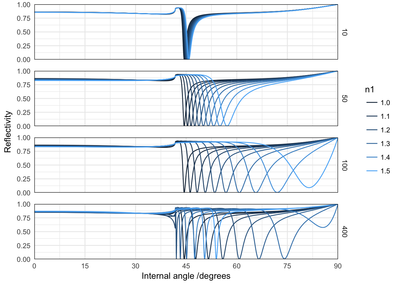

For an optical thickness approaching \(\lambda / 2\), a new reflectivity dip appears, that is associated with the excitation of a guided mode. It is sharper than the standard SPP mode, because the modal field is mostly located in the dielectric layer.